In general, thermal analysis is a very convenient way to study the kinetics of thermally activated solid reactions, and experiments involving thermally activated solid reactions typically occur under nonisothermal conditions. The experimental data analysis obtained under non-isothermal conditions includes a temperature integral, also called the Arrhenius integral, which is one of the integrals that belong to many interesting integrals that are important in engineering and have no analytical solution. There are many different approximations that can be applied to the processing of thermogravimetric analysis data, since there is no standard way to calculate the temperature integral. Many approximations of the temperature integral that are important to use determine the kinetic parameters, especially the activation energy, which are typically divided into two categories: exponential and rational approximations. In order to evaluate the accuracy of various approximations of the temperature integral, we consider several certain continuous intervals. When choosing an approximation of the temperature integral needed to analyze the experimental data, it is necessary to analyze the accuracy at different temperature intervals of the approximation and use the appropriate one. We present new rational, irrational and continued fractional approximations together with approximations of the temperature integral presented in several literatures and calculate the relative errors of their activation energies.
| Published in | Science Journal of Applied Mathematics and Statistics (Volume 14, Issue 3) |
| DOI | 10.11648/j.sjams.20261403.11 |
| Page(s) | 71-78 |
| Creative Commons |
This is an Open Access article, distributed under the terms of the Creative Commons Attribution 4.0 International License (http://creativecommons.org/licenses/by/4.0/), which permits unrestricted use, distribution and reproduction in any medium or format, provided the original work is properly cited. |
| Copyright |
Copyright © The Author(s), 2026. Published by Science Publishing Group |
Temperature Integral, Solid-state Reactions, Nonisothermal Conditions, Approximation, Activation Energy
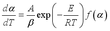 (1)
(1)  (0 <
(0 <  <1) is the fractional conversion,
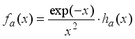
  (K/min) the heating rate, E (kJ/mol) the activation energy, A (min-1) the preexponential factor, R the gas constant, T (K) the absolute temperature, specific form of
  represents the hypothesized model of the reaction mechanism.
 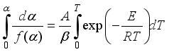 (2)
(2) 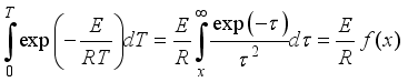 (3)
(3) 
 (4)
(4)  (5)
(5)  (6)
(6)  (7)
(7)  (8)
(8)  (9)
(9)  (10)
(10) Name | lnpa(x) | ε1 | ε2 | ||
|---|---|---|---|---|---|
b | K | a | |||
Doyle | -5.3308 | 0 | 1.0516 | 15.39 | 0.91 |
TLZW | -0.37773896 | 1.8946610 | 1.00145033 |
|
|
Cai–Liu [7] | -0.460120828342246 | 1.86847901883656 | 1.00174866236974 |
|
|
 (11)
(11)  (12)
(12)  (13)
(13) 

Name | Approximation | N | n | ε1 | ε2 |
|---|---|---|---|---|---|
FJG [ 19] | 1 | 0 | 0 | 0.65 | 0.19 |
Coats–Redfern |
| 1 | 1 |
|
|
Cai |
| 2 | 1 |
|
|
Urbanovici–Segal II |
| 3 | 2 |
|
|
Senum–Yang I |
| 3 | 2 |
|
|
Ji |
| 4 | 2 |
|
|
Senum-Yang III |
| 7 | 4 |
|
|
|
| 8 | 4 |
|
|
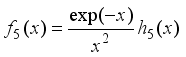
h5 |
| 9 | 5 |
|
|
h6 |
| 11 | 6 |
|
|
h7 |
| 13 | 7 |
|
|
Name | Approximation | ε1 | ε2 |
|---|---|---|---|
Balarin |
|
|
|
hr2 |
|
|
|
hr5 |
|
|
|
Name | Approximation | ε1 | ε2 |
|---|---|---|---|
hc1 |
|
|
|
hc2 |
|
|
|
 ,(14)
,(14)  .(15)
.(15) x | FJG [ 19] | Coats–Redfern | Cai | Urbanovici–Segal II | Senum–Yang I | Ji | Senum-Yang III | |
|---|---|---|---|---|---|---|---|---|
0.5 |
|
|
|
|
|
|
|
|
2 |
|
|
|
|
|
|
|
|
5 |
|
|
|
|
|
|
|
|
10 |
|
|
|
|
|
|
|
|
15 |
|
|
|
|
|
|
|
|
20 |
|
|
|
|
|
|
|
|
25 |
|
|
|
|
|
|
|
|
30 |
|
|
|
|
|
|
|
|
40 |
|
|
|
|
|
|
|
|
45 |
|
|
|
|
|
|
|
|
50 |
|
|
|
|
|
|
|
|
55 |
|
|
|
|
|
|
|
|
60 |
|
|
|
|
|
|
|
|
80 |
|
|
|
|
|
|
|
|
100 |
|
|
|
|
|
|
|
|
x | Balarin | h5 | h6 | h7 | hr2 | hr5 | hc1 | hc2 |
|---|---|---|---|---|---|---|---|---|
0.5 |
|
|
|
|
|
|
| |
2 |
|
|
|
|
|
|
|
|
5 |
|
|
|
|
|
|
|
|
10 |
|
|
|
|
|
|
|
|
15 |
|
|
|
|
|
|
| |
20 |
|
|
|
|
|
| ||
25 |
|
|
|
|
|
| ||
30 |
|
|
|
|
|
| ||
40 |
|
|
|
|
|
| ||
45 |
|
|
|
|
|
| ||
50 |
|
|
|
|
|
| ||
55 |
|
|
|
|
|
| ||
60 |
|
|
|
|
|
| ||
80 |
|
|
|
|
|
| ||
100 |
|
|
|
|
|
|
x | FJG [ 19] | Coats–Redfern | Cai | Urbanovici–Segal II | Senum–Yang I | Ji | Senum-Yang III | |
|---|---|---|---|---|---|---|---|---|
0.5 |
|
|
|
|
|
|
| |
2 |
|
|
|
|
|
|
| |
5 |
|
|
|
|
|
|
| |
10 |
|
|
|
|
|
| ||
15 |
|
|
|
|
|
| ||
20 |
|
|
|
|
|
| ||
25 |
|
|
|
|
|
| ||
30 |
|
|
|
|
|
| ||
40 |
|
|
|
|
|
| ||
45 |
|
|
|
|
|
| ||
50 |
|
|
|
|
|
| ||
55 |
|
|
|
|
|
| ||
60 |
|
|
|
|
|
| ||
80 |
|
|
|
|
|
| ||
100 |
|
|
|
|
|
|
x | Balarin | h5 | h6 | h7 | hr2 | hr5 | hc1 | hc2 |
|---|---|---|---|---|---|---|---|---|
0.5 |
|
|
|
|
|
|
| |
2 |
|
|
|
|
|
|
|
|
5 |
|
|
|
|
|
|
|
|
10 |
|
|
|
|
|
|
|
|
15 |
|
|
|
|
|
|
| |
20 |
|
|
|
|
|
|
| |
25 |
|
|
|
|
| |||
30 |
|
|
|
|
|
| ||
40 |
|
|
|
|
|
| ||
45 |
|
|
|
|
|
| ||
50 |
|
|
|
|
|
| ||
55 |
|
|
|
|
|
| ||
60 |
|
|
|
|
|
|
| |
80 |
|
|
|
|
| |||
100 |
|
|
|
|
|
|
TGA | Thermogravimetric Analysis |
| [1] | Hammam, M., Abdel-Rahim, M. Hafiz, M., Abu-Sekly A., New combination of noil-isothermal kinetics-revealing methods. J Therm Anal Calorim [Internet]. 2017, 128(3), 1391-405. |
| [2] | Sstk, J., Are nonisotkermal kinetics fearing historical Newton’s cooling law, or are just afraid of inbuilt complications due to undesirable thermal inertial. J Therm Anal Calorim. 2018, 134(3), 1385-93. |
| [3] | Burnham, A. K., Use and misuse of logistic equations for modeling chemical kinetics. J Therm Anal Calorim. 2017, 127(1), 1107-16. Available from: |
| [4] | Cai, J., Wu, W., Liu R., Isoconversional kinetic analysis of complex solid-state processes: Parallel and successive reactions. Ind Eng Chem Res [Internet]. 2012, 51(49), 16157-61. |
| [5] | Mortici, C., A continued fraction approximation of the gamma function. J. Math. Anal. Appl. 402(2013), 405–410. |
| [6] | Chen, C.-P., A more accurate approximation for the gamma function. J. Num. The. 164(2016) 417–428. |
| [7] | Nemes, G., Approximations for the higher order coefficients in an asymptotic expansion for the Gamma function. J. Math. Anal. Appl. 396 (2012), 417–424. |
| [8] | Prez-Maqueda, L. A., Criado, J. M., J. Therm. Anal. Calorim. 60(2000), 909. |
| [9] | Zhang, X., Applications of Kinetic Methods in Thermal Analysis: A Review. Eng. Sci., 2021, 14, 1–13. |
| [10] | Budrugeac, P., An iterative model-free method to determine the activation energy of non-isothermal heterogeneous processes. Thermochimica Acta, 2010, 511, 8–16. |
| [11] | Mu, X., Xuanjun W., Xiangxuan L., Youzhi Z., Thermal Decomposition Performance of Unsymmetrical Dimethylhydrazine (UDMH) Oxalate. PEP, 2012, 37, 316-319. |
| [12] | Chen, N. H., Jin, S., Li, S., Jing, L., Jiang, B., Ji, Z., Qinghai, J. S., Thermolysis, nonisothermal decomposition kinetics, calculated detonation velocity and safety assessment of dihydroxylammonium 5, 5′-bistetrazole-1, 1′-diolate. J. Therm Anal Calorim, 2016, 126, 473–480. |
| [13] | Yi, J. H., Zhao, F. Q., Hong, W. L., Xu, S. Y., Hu, R. Z. Chen, Z. Q. Zhang, L. Y., Effects of Bi-NTO complex on thermal behaviors, nonisothermal reaction kinetics and burning rates of NG/TEGDN/NC propellant. Journal of Hazardous Materials, 2010, 176, 257–261. |
| [14] | Chen, R. Y., Li, Q. W., Xu, X. K. Zhang, D. D., Hao, R. L., Combustion characteristics, kinetics and thermodynamics of Pinus Sylvestris pine needle via non-isothermal thermogravimetry coupled with model-free and model-ftting methods. Case Studies in Thermal Engineering, 2020, 22, 100756. |
| [15] | Yasnó, J. P., Conconi, S., Visintin, A., Suárez, G., Non-isothermal reaction mechanism and kinetic analysis for the synthesis of monoclinic lithium zirconate (m-Li2ZrO3) during solid-state reaction. Journal of Analytical Science and Technology. 2021, 12-15. |
| [16] | Carrero-Mantilla, J. I., Rojas-Gouzlez, A. F., Calculation of the temperature integrals used in the processing of thermogravimetric analysis data, 2019, Vol. 21 No. 2. |
| [17] | Deng., C., Cai., J., Liu, R., Kinetic analysis of solid-state reactions: Evaluation of approximations to temperature integral and their applications. Solid State Sciences 11(2009) 1375–1379. |
| [18] | Tang, W., Liu, Y., Zhang, H., Wang, C., Thermochim. Acta 408(2003) 39. |
| [19] | Ernesto Fischer, P., Chon Shin J., Shyam, S., Gokalgandhi, Ind. Eng. Chem. Res. 26(1987) 1037. |
APA Style
Chol, K. H., Il, R. K. (2026). Evaluation of Some Approximations of the Temperature Integral Used in Kinetic Analysis of Solid-state Reactions. Science Journal of Applied Mathematics and Statistics, 14(3), 71-78. https://doi.org/10.11648/j.sjams.20261403.11
ACS Style
Chol, K. H.; Il, R. K. Evaluation of Some Approximations of the Temperature Integral Used in Kinetic Analysis of Solid-state Reactions. Sci. J. Appl. Math. Stat. 2026, 14(3), 71-78. doi: 10.11648/j.sjams.20261403.11
@article{10.11648/j.sjams.20261403.11,
  author = {Kim Hyon Chol and Ri Kwang Il},
  title = {Evaluation of Some Approximations of the Temperature Integral Used in Kinetic Analysis of Solid-state Reactions},
  journal = {Science Journal of Applied Mathematics and Statistics},
  volume = {14},
  number = {3},
  pages = {71-78},
  doi = {10.11648/j.sjams.20261403.11},
  url = {https://doi.org/10.11648/j.sjams.20261403.11},
  eprint = {https://article.sciencepublishinggroup.com/pdf/10.11648.j.sjams.20261403.11},
  abstract = {In general, thermal analysis is a very convenient way to study the kinetics of thermally activated solid reactions, and experiments involving thermally activated solid reactions typically occur under nonisothermal conditions. The experimental data analysis obtained under non-isothermal conditions includes a temperature integral, also called the Arrhenius integral, which is one of the integrals that belong to many interesting integrals that are important in engineering and have no analytical solution. There are many different approximations that can be applied to the processing of thermogravimetric analysis data, since there is no standard way to calculate the temperature integral. Many approximations of the temperature integral that are important to use determine the kinetic parameters, especially the activation energy, which are typically divided into two categories: exponential and rational approximations. In order to evaluate the accuracy of various approximations of the temperature integral, we consider several certain continuous intervals. When choosing an approximation of the temperature integral needed to analyze the experimental data, it is necessary to analyze the accuracy at different temperature intervals of the approximation and use the appropriate one. We present new rational, irrational and continued fractional approximations together with approximations of the temperature integral presented in several literatures and calculate the relative errors of their activation energies.},
 year = {2026}
}
TY  - JOUR
T1  - Evaluation of Some Approximations of the Temperature Integral Used in Kinetic Analysis of Solid-state Reactions
AU  - Kim Hyon Chol
AU  - Ri Kwang Il
Y1  - 2026/06/12
PY  - 2026
N1  - https://doi.org/10.11648/j.sjams.20261403.11
DO  - 10.11648/j.sjams.20261403.11
T2  - Science Journal of Applied Mathematics and Statistics
JF  - Science Journal of Applied Mathematics and Statistics
JO  - Science Journal of Applied Mathematics and Statistics
SP  - 71
EP  - 78
PB  - Science Publishing Group
SN  - 2376-9513
UR  - https://doi.org/10.11648/j.sjams.20261403.11
AB  - In general, thermal analysis is a very convenient way to study the kinetics of thermally activated solid reactions, and experiments involving thermally activated solid reactions typically occur under nonisothermal conditions. The experimental data analysis obtained under non-isothermal conditions includes a temperature integral, also called the Arrhenius integral, which is one of the integrals that belong to many interesting integrals that are important in engineering and have no analytical solution. There are many different approximations that can be applied to the processing of thermogravimetric analysis data, since there is no standard way to calculate the temperature integral. Many approximations of the temperature integral that are important to use determine the kinetic parameters, especially the activation energy, which are typically divided into two categories: exponential and rational approximations. In order to evaluate the accuracy of various approximations of the temperature integral, we consider several certain continuous intervals. When choosing an approximation of the temperature integral needed to analyze the experimental data, it is necessary to analyze the accuracy at different temperature intervals of the approximation and use the appropriate one. We present new rational, irrational and continued fractional approximations together with approximations of the temperature integral presented in several literatures and calculate the relative errors of their activation energies.
VL  - 14
IS  - 3
ER  -
Faculty of Mathematics, Kim Il Sung University, Pyongyang, DPR Korea
Information