Combustible Ethanol-Gasoline Blend for Reduced Carbon Monoxide Emission

Shehu Sule Aboje; Toyin Olabisi Odutola

doi:doi:10.11648/j.pse.20261001.12

Research Article |

| Peer-Reviewed

Combustible Ethanol-Gasoline Blend for Reduced Carbon Monoxide Emission

Shehu Sule Aboje

, Toyin Olabisi Odutola^*

Published in Petroleum Science and Engineering (Volume 10, Issue 1)

Received: 19 January 2026 Accepted: 5 February 2026 Published: 27 February 2026

Views: Downloads:

Download PDF

Share This Article

Twitter
Linked In
Facebook

Abstract

This study presents the emission profiles and combustion characteristics of ethanol-gasoline blends in internal combustion engines with the goal of reducing environmental impact and increasing efficiency in Nigeria. The goal of the project is to assess the exhaust emissions and combustion properties of different ethanol-gasoline blends in internal combustion engines to increase efficiency and lessen environmental effect. Palm sap was used to make ethanol, which was then combined with gasoline from the Dangote Refinery's MRS filling station to create mixes E5 (95% gasoline), E10 (90% gasoline), E15 (85% gasoline), and E20 (80% gasoline). To establish performance criteria for these blends, known concentrations of n-heptane were added. The following physicochemical investigations were performed: density and specific gravity, octane rating, flash point, boiling point range, Reid Vapor Pressure (RVP), and heating value. In addition, engine performance was measured at different engine torque levels (3.0, 3.5, 4.0, and 4.5 kW) to compute the corresponding speed, brake specific energy consumption (BSEC), brake specific fuel consumption (BSFC), fuel equivalent power (FEP), and brake thermal efficiency (BTE). Emission tests were also conducted to evaluate gas emissions in compliance with environmental standards and regulations. Blends of ethanol and gasoline, particularly E15 and E20, provide promising ways to reduce air pollution in cities, boost engine torque, and use renewable resources that are harvested locally. In addition to providing helpful information for more general policy, technical, and scholarly conversations, this study highlights the role that ethanol plays in Nigeria's low-carbon energy transition.

Published in	Petroleum Science and Engineering (Volume 10, Issue 1)
DOI	10.11648/j.pse.20261001.12
Page(s)	17-36
Creative Commons	This is an Open Access article, distributed under the terms of the Creative Commons Attribution 4.0 International License (http://creativecommons.org/licenses/by/4.0/), which permits unrestricted use, distribution and reproduction in any medium or format, provided the original work is properly cited.
Copyright	Copyright © The Author(s), 2026. Published by Science Publishing Group

Keywords

Ethanol-Gasoline, n-Heptane, Blends, Engine, Emission, Gasoline Engine, Renewable Energy

1. Introduction

Automobile tailpipe emissions are a major source of air pollution and greenhouse gases, highlighting the urgent need for renewable fuel alternatives. The rapid increase in global vehicle populations has elevated atmospheric concentrations of CO₂, SO₂, and H₂S, adversely affecting human health, air quality, and ecosystem stability

[1]

. Exposure to these emissions can cause respiratory inflammation and tissue damage, while secondary atmospheric reactions contribute to smog formation and ozone layer depletion. CO₂, in particular, exerts the greatest influence on global warming, accelerating sea-level rise and disrupting ecological balance

[2]

. In response, international conventions, agreements, and protocols have been established to legally bind nations to implement measures that mitigate environmental degradation. Nigeria, a signatory to these agreements

[3]

, mandates fuel blends of 90% gasoline with 10% ethanol and up to 20% biodiesel, enforced by the Nigeria National Petroleum Corporation (NNPC)

[4]

. Despite policy frameworks and incentives in place since 2007, Nigeria has yet to develop a domestic biofuel industry, continuing to rely heavily on imported fossil fuels. This underutilization persists despite the country’s abundant agricultural resources suitable for biofuel production, representing a significant missed opportunity to reduce emissions and advance sustainable energy goals.

Adding ethanol to gasoline offers a practical approach to address these challenges. Ethanol’s higher octane number improves combustion efficiency, with a 10% blend increasing the research octane number by ~5 units and reducing knocking and pre-ignition

[5]

. Ethanol–gasoline and ethanol–n-heptane blends can also lower pollutant emissions and fuel costs. This study examines their effects on engine performance, combustion characteristics, and emission profiles, providing critical insights for Nigerian policymakers, the automotive industry, and vehicle owners. While a full transition to renewable fuels may be gradual, strategic adoption of ethanol blends presents a viable pathway to enhance engine efficiency and reduce environmental impacts.

Numerous studies have investigated the effects of ethanol–gasoline blended fuels on internal combustion engine performance and exhaust emissions. In addition, the use of oxygenated additives such as methyl tertiary butyl ether (MTBE) has been reported to enhance engine efficiency and reduce emissions associated with incomplete combustion

[6]

. Experimental evaluations using both neat gasoline and gasoline–MTBE blends (M5 and M10) on a four-cylinder, 1817 cc engine revealed that MTBE-blended fuels produced higher brake thermal efficiency (BTE) and brake-specific fuel consumption (BSFC). However, these blends also resulted in increased CO₂ and NOₓ emissions, alongside reduced hydrocarbon (HC) and carbon monoxide (CO) emissions. The influence of ethanol addition on gasoline engine performance and exhaust emissions has also been examined across varying ethanol volume fractions, including 10% (E10), 20% (E20), and 30% (E30), using a four-stroke, single-cylinder engine

[7]

. The results demonstrated that increasing the alcohol blend ratio generally led to improved engine performance and cleaner exhaust emissions. Furthermore, studies on the combustion and emission characteristics of ethanol–n-butanol blends in a single-cylinder heavy-duty engine

[8]

indicated that alcohol-based blends significantly reduced soot emissions, particularly at medium load conditions. Compared with conventional fuels, ethanol was found to require higher temperatures for auto-ignition. Overall, these findings emphasize the importance of optimizing additive combinations and engine operating conditions to achieve reduced particulate emissions without compromising combustion efficiency.

From the literature survey, with little or no modifications, ethanol–gasoline blended fuels can be used effectively in combustible engine. The ratio of ethanol formulation in gasoline alters the fuel's combustibility qualities significantly. Ethanol has a higher octane rating compared to gasoline, and every 10% increase in ethanol raises the blend's research octane number by 5 units, potentially increasing engine power

[5]

. A higher octane rating promotes more efficient combustion by lowering pre-ignition and knocking. Compared to gasoline, ethanol has different combustion characteristics. It is safer to carry and store because of its higher auto-ignition temperature and flashpoint. Additionally, alcohol has a far higher latent heat of evaporation, which leads to higher volumetric efficiency and lower input manifold temperatures. But because alcohol has a lower heating value than gasoline, more alcohol fuel—roughly 1.5–1.8 times more—is needed to provide the same amount of energy

[9]

. In addition, the stoichiometric air-fuel ratio (AFR) of alcohol is two-thirds to half that of gasoline. This indicates that a small amount of air is needed for complete combustion when alcohol is utilized as fuel. Compared to gasoline, ethanol requires a lower stoichiometric air/fuel ratio because it is an oxygenated fuel.

n-Heptane (C₇H₁₆) is a linear alkane widely used as a reference compound in fuel combustion research due to its well-characterized oxidation kinetics and low auto-ignition resistance. The lower bound of knock resistance in spark-ignition engines is represented by n-heptane, one of the two main reference fuels used for octane rating, which has an assigned research octane number (RON)

[10]

. Although pure n-heptane is rarely found in practical applications, the compound is commonly used in surrogate fuel mixtures (such as toluene/n-heptane or iso-octane/n-heptane blends) to simulate the combustion behaviour of commercial gasoline in experimental and computational studies

[11]

. The combustion characteristics of n-heptane differ significantly from those of oxygenated fuels like ethanol. n-Heptane exhibits two-stage ignition behaviour under engine-relevant conditions, with low-temperature chemistry playing a crucial role in its auto-ignition

[12]

. This work is required to completely comprehend the effects of ethanol concentrations in combination with n-heptane on emissions and engine performance. Even though ethanol-gasoline mixes enhance engine performance and emissions, a full understanding of the combustion and emission mechanisms is still required.

2. Materials and Methods

Ethanol was produced in Nukpo Yeghe, Gokana Local Government Area in Rivers State, Nigeria. This region, situated in the humid tropics of the Niger Delta, experiences high ambient temperatures (28–32°C) and relative humidity (70–85%), which promote microbial activity and fermentation. These conditions create an ideal environment for the natural production of ethanol from palm sap. Laboratory analyses were performed at Spectral Laboratory Services in Kaduna State.

2.1. Raw Material

The primary sources of raw materials for this investigation were n-heptane bought from a local Kaduna seller, gasoline from MRS gas station, refined petroleum product from Dangote Refinery in Lagos, and fresh palm sap from mature Elaeis guineensis trees. To avoid contamination, sterile collection containers were used, and clean, sharp instruments were used to create incisions in the inflorescence in order to extract the sap.

2.1.1. Microorganism

Fermentation was initiated by naturally occurring wild yeast (Saccharomyces cerevisiae) discovered in palm sap, with no exogenous microbial inoculants used.

2.1.2. Chemicals and Reagents

Deionized Water

Benzoic Acid

Pure Oxygen (99.99%)

2.2. Bio-ethanol Production Process

In Nukpo Yeghe, Gokana LGA, Rivers State, bio-ethanol was made using palm sap (Elaeis guineensis) that was readily available in the area. The method began with the careful extraction of sap from fully grown palm trees. Removing a few leaves from the top of the stem is the first stage in tapping. Even when the stem is shaved into a cone shape, the terminal bud and a few fronds are kept intact to allow the palm to survive. To channel the sap flow from the cone to a container, a spout is connected to a canal that is cut around the base of the cone. The cone is first covered to prevent drying out in the sun, and then it is recut to remove the dry surface and allow the sap to flow in. Fermentation was initiated naturally by the wild yeast (Saccharomyces cerevisiae) present in the sap. The mixture was left to ferment for 24 hours at room temperature (28–32°C). During this time, the sugars were transformed into carbon dioxide and ethanol, as evidenced by bubbling and a pH drop to about 4.0. A two-step distillation procedure was used to extract the fermented sap. The first step involved heating the liquid to 78–82°C, the boiling point of ethanol, in a stainless-steel distillation drum. A water-cooled steel pipe system was used to condense the resultant vapors, producing a liquid with 40–60% ethanol. Using a hydrometer (ASTM D5501), a second distillation was carried out to attain a greater purity of ≥95%. To stop moisture absorption, the finished product was kept in sealed containers.

Download: Download full-size image

Figure 1. Ethanol production.

2.3. Preparation of Ethanol-Gasoline Blends with n-Heptane

Ethanol–gasoline blends (1 L each) were prepared on a volumetric basis in accordance with ASTM D4814 fuel blending practice. The required volumes of anhydrous ethanol, base gasoline, and n-heptane were calculated according to the specified blend ratios. Base gasoline and ethanol were first introduced into a clean, dry, and airtight container and mixed to obtain a uniform gasohol base. n-Heptane was subsequently added in measured increments under continuous agitation to ensure homogeneous distribution throughout the blend. Mixing was continued for 30 min to achieve complete miscibility and uniform fuel properties. The finished blends were transferred to sealed, clearly labeled metal containers to minimize evaporative losses and contamination and stored at ambient laboratory conditions (28–30°C). The prepared fuels were designated according to ethanol volume fraction (e.g., E0, E10, E15, E20) and were subjected to physicochemical property testing to verify compliance with performance and safety requirements specified in ASTM D4814.

Download: Download full-size image

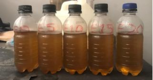
Figure 2. Ethanol-gasoline blends.

Table 1. Ethanol-gasoline blends.

Blend Code	Ethanol Volume (mL)	Petrol Volume (mL)	Ethanol % (v/v)
E0	0	1000	0%
E5	50	950	5%
E10	100	900	10%
E15	150	850	15%
E20	200	800	20%
E100	1000	0	100%

Table 2. n- Heptane Blend.

Blend Code	n- Heptane Volume (mL)	Gasohol Volume (mL)	n- Heptane% (v/v)
E0	0	1000	0%
E5	50	950	5%
E10	100	900	5%
E15	150	850	15%
E20	200	800	20%
E100	0	0	0%

2.4. Properties of the Fuel

2.4.1. Determination of the Density

Fuel density was determined in accordance with ASTM D129–12b (2017) using the hydrometer method. Each sample was conditioned to a specified test temperature, after which a test portion was transferred into a hydrometer cylinder pre-equilibrated to the same temperature. An appropriate hydrometer was then carefully immersed in the sample and allowed to stabilize under thermal equilibrium. The hydrometer scale reading and corresponding sample temperature were recorded. The observed hydrometer reading was corrected to the reference temperature using standard petroleum measurement tables, and any applicable hydrometer corrections were applied. Density values were reported using the corrected hydrometer reading to the nearest 0.1 kg·m⁻³. Each measurement was repeated three times to ensure precision and accuracy.

2.4.2. Viscosity Measurement

Kinematic viscosity, defined as the ratio of dynamic viscosity to density, was determined using a Brookfield digital rotational viscometer. Prior to measurement, each sample was heated in a thermostatically controlled oil bath to the required test temperature. The viscometer spindle was then immersed in the sample and rotated at a selected speed. Viscosity and operating temperature were displayed digitally upon stabilization of the rotational torque. Each viscosity measurement was performed three times under identical conditions, and the mean value was reported to ensure precision and repeatability.

2.4.3. Distillation Characteristics (ASTM D86–23)

Distillation characteristics were determined in accordance with ASTM D86–23. A 100 mL sample was charged into a 250 mL two-neck round-bottom distillation flask fitted with a condenser and thermometer. The assembly was placed on a temperature-controlled heating mantle, and heat input was regulated to achieve standard distillation rates. Temperatures corresponding to 10%, 30%, 70%, and 90% volume recovered were recorded. Each distillation test was conducted three times, and average values were used for analysis.

2.4.4. Cloud Point and Pour Point

Cloud point and pour point were determined using a standardized cooling procedure. Each sample was poured into a test tube to a specified level, sealed, and fitted with a thermometer before placement in the cooling apparatus. The sample was periodically inspected during cooling. The cloud point was recorded as the temperature at which a visible cloud or haze first appeared, while the pour point was defined as the lowest temperature at which the sample exhibited flow. All measurements were repeated three times to ensure precision and reproducibility.

2.4.5. Flash Point and Fire Point (ASTMD 93)

Flash point and fire point were measured using a Pensky–Martens closed-cup apparatus in accordance with ASTM D93. Approximately 50 mL of sample was introduced into a clean, dry test cup, which was then secured in the apparatus and equipped with a thermometer and mechanical stirrer. The sample was heated at a controlled rate, and a test flame was applied at 5 s intervals. The flash point was recorded as the lowest temperature at which the vapor ignited momentarily, while the fire point was defined as the temperature at which sustained combustion occurred. The apparatus was cleaned and dried between tests. Each measurement was repeated times, and mean values were reported.

2.4.6. Heat of Vaporization (ASTMD 93)

The gross heat of combustion of the fuel samples was determined using an oxygen bomb calorimeter (Model 6100, Parr Instrument Co., Moline, IL) in accordance with ASTM D2382–88. Prior to testing, the calorimeter was calibrated using a known mass of standard benzoic acid with a certified heat of combustion of 26.453 kJ·g^-1. Approximately 0.1 g of each fuel sample and 1 mL of deionized water were introduced into the calibrated adiabatic bomb. The ignition electrodes were connected with a Chromel (Ni–Cr) wire positioned in contact with the sample. The bomb was sealed, purged twice with high-purity oxygen (99.99%) at 0.5 MPa, and subsequently charged to an oxygen pressure of 2.0 MPa. The assembled bomb was immersed in an insulated calorimeter jacket containing 2 L of water, which was continuously stirred to ensure uniform temperature distribution. Sample ignition was initiated electrically, and complete combustion occurred under constant-volume, high-pressure oxygen conditions. The temperature rise was recorded automatically, and the gross heat of combustion was computed and displayed in kJ·kg^-1. Each measurement was repeated three times under identical conditions, and the average value was reported to ensure precision and repeatability.

2.4.7. Boiling Point Determination

The boiling point of each fuel sample was determined using the capillary tube method. A sealed glass capillary tube was inverted and immersed in the liquid sample, which was then heated gradually. As temperature increased, the vapor pressure of the sample rose, displacing the trapped air within the capillary and producing a continuous stream of bubbles. Upon cooling, liquid re-entered the capillary when the vapor pressure equaled atmospheric pressure. The boiling point was recorded as the sample temperature at this equilibrium condition. Each measurement was repeated three times under identical conditions, and the average value was reported to ensure repeatability.

2.4.8. Octane-Cetane Number (ASTMD 613)

The octane and cetane characteristics of the gasoline and blended fuels were evaluated using an Octane Meter IM. Approximately 10 mL of each sample was transferred into a clean cuvette, after which the probe spindle was immersed in the fuel and allowed to rotate. Following a stabilization period of 30 s, the research octane number (RON) and motor octane number (MON) were displayed and recorded. Cetane-related combustion quality indices were obtained in accordance with ASTM D613 principles. Each measurement was conducted three times, and mean values were used for analysis.

2.4.9. Reid Vapor Pressure (RVP) Determination

Reid vapor pressure was determined using a standard vapor pressure apparatus. Each sample was introduced into the test cuvette to approximately 70% capacity and conditioned in an ice–water bath at 1°C for 30 min. The cuvette was then connected to the vaporization chamber fitted with a calibrated pressure gauge and shaken vigorously before being returned to the ice bath for at least 2 min. Subsequently, the assembled apparatus was immersed in a water bath maintained at 37.8°C. After thermal equilibrium was achieved, the device was removed and inverted five times, and the stabilized pressure reading was recorded as the RVP. All RVP measurements were repeated three times to ensure precision and reproducibility.

2.4.10. Higher Heating Value (HHV) Determination

The higher heating value (HHV) of the fuel samples was determined using an oxygen bomb calorimeter (Model 6100, Parr Instrument Co., Moline, IL). Prior to testing, the calorimeter was calibrated by combusting a known mass of standard benzoic acid with a certified heat of combustion of 26.453 kJ·g^-1. Fuel samples were combusted under constant-volume conditions, and the resulting temperature rise was used to calculate the calorific value, expressed in kJ·kg^-1. Each HHV measurement was performed three times, and the average value was reported.

2.5. Engine Test

A four-cylinder Honda gasoline engine rated at 3 kW (4.08 hp) and operating at 230 V and 50 Hz was used. The engine was coupled to a Froude hydraulic dynamometer for load application and torque measurement. Fuel consumption was measured using a calibrated fuel tank (±0.5 accuracy) via a volumetric method and converted to mass flow rate. Engine speed, temperature, and torque were monitored using a tachometer, thermocouple, load cells, and an instrumentation unit. Engine load was varied by regulating water flow into the dynamometer following preliminary stabilization and calibration tests. Brake power (BP), brake specific fuel consumption (BSFC), brake specific energy consumption (BSEC), brake thermal efficiency (BTE), fuel-equivalent power (FEP), and fuel consumption rate (FC) were calculated using Eqs. (1)–(6). Each test condition was repeated three times to ensure repeatability and data reliability.

Mf = \frac{m}{t} \times \frac{p}{t}

(1)

Pf = Hg \times Mf

(2)

BP = \frac{NT}{14300}

(3)

BSFC = \frac{Mf}{BP}

(4)

BESEC = BSFC \times Hg

(5)

nbt h = \frac{BP}{Mf} ×Hg×100

(6)

2.6. Emission Test

After powering on, the apparatus (Figure 3) was allowed to initialize for 60 s, followed by a stabilization period of 5 min. To ensure proper initialization, the analyzer was connected to a computer via USB, and an airtight rubber tube was secured to the gas sampling point, either from the gas bag or the gas vessel outlet. Gas flow to the sensor was activated for 60 s by opening the gas valve, allowing the signal to stabilize. Measurements were recorded once the analyzer displayed the complete gas sample response, and flow was continuously monitored to ensure reliable sampling. Data were logged using the analyzer’s save function and subsequently exported via the connected software for processing. After completion of each measurement, the system was purged with nitrogen to remove residual gas, the gas bag valve was closed, and the sampling tube was disconnected before shutdown. All measurements were performed in triplicate to ensure repeatability, and the recorded emissions were compared against relevant performance standards.

Download: Download full-size image

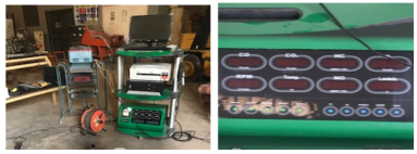
Figure 3. Gas Analyzer.

3. Results and Discussion

This study focuses on ethanol-gasoline mixes, offering valuable insights into how the physicochemical properties of ethanol impact engine performance and emissions, whereas the original scope covered n-heptane blends. In this study, efficiency metrics like brake-specific fuel consumption (BSFC) and thermal efficiency, along with emissions of particulate matter (PM), nitrogen oxides (NOx), carbon monoxide (CO), and unburned hydrocarbons (HC), are examined to identify trade-offs and opportunities for ethanol blend optimization. To highlight both continuities and novel contributions, the findings are placed within the framework of recent literature, setting the stage for further study and real-world applications.

3.1. Physicochemical Analysis

Table 3. Thermal and Physical Properties of the Gasoline-Ethanol Blends.

PARAMETERS	E0	E5	E10	E15	E20	E100
THERMAL PROPERTIES
Density (mg/l)	0.7720	0.7761	0.7836	0.7942	0.7987	0.9345
Specific gravity	0.7894	0.7936	0.8013	0.8121	0.8167	0.9556
THERMAL PROPERTIES
Reid vapor pressure (psi)	9.3	9.9	10.4	11.2	11.0	4.4
Research octane number	119	121	123	126	129	135
Motor octane number	98	99	100	101	103	107
Heat of vaporization (mj/kg)	34.2525	33.9247	33.7063	33.6992	33.5078	28.5808
Stoichiometric airflow ratio
Flash point (^oc)	NA	NA	NA	NA	33.2	38.6
Boiling point (^oc)	34.2	36.1	39.7	41.1	44.3	83.3

The results in Table 3 indicate that the specific gravity and density of the blends increase linearly with the percentage of ethanol. It has been observed that ethanol's density influences spray dynamics, necessitating improved injector designs to avoid incomplete combustion. Typically, energy content per volume increases with density, which can enhance fuel economy and affect the emission profiles of vehicles using bioethanol. Overall, the findings suggest that an E20 blend could potentially reduce exhaust emissions while improving engine performance.

E15 exhibits the best cold start and vaporization profile among all blends, achieving a peak Reid vapor pressure of 11.2 psi. In contrast, E100 has a much lower RVP of 4.4 psi, which could lead to difficult cold starts in temperate climates. E20’s modest decrease to 11.0 psi may result in slightly diminished low-temperature drivability. The initial rise in RVP from E0 to E15 is attributed to lighter hydrocarbons in gasoline, such as butane and pentane, which enhance cold-start performance but also increase evaporative emissions. The subsequent decline in RVP from E20 to E100 is due to ethanol's lower volatility, which re duces the risk of vapor lock but can create cold-start issues in colder environments. While blends E20–E100 are more suitable for tropical climates like Nigeria, where higher ambient temperatures help mitigate vaporization concerns, E10–E15 is preferable for temperate regions with harsh winters. This dual behavior highlights the importance of optimizing fuel blends for specific regional conditions. As ethanol content increases, both the Research Octane Number (RON) and Motor Octane Number (MON) rise linearly, moving from 119 to 135 (RON) and 98 to 107 (MON), respectively. At E15, octane performance (RON = 126, MON ≈ 101) offers a significant anti-knock margin over E10 (RON ≈ 123) while avoiding the diminishing returns and calibration complexities associated with higher ethanol concentrations like E20 and E100. This allows for slight improvements in ignition timing or compression ratios without necessitating major engine modifications.

Despite ethanol's well-established high latent heat (~840 kJ/kg compared to gasoline's ~350 kJ/kg), the reported heat of vaporization decreases with ethanol content (34.25 MJ/kg for E0 to 28.58 MJ/kg for E100). The LHV of ethanol (~26.8 MJ/kg) compared to gasoline (~44.4 MJ/kg) explains why engine tests show higher Brake-Specific Fuel Consumption (BSFC), since more fuel is needed to maintain power output. Lastly, despite the apparent anomaly in the heat of vaporization data, the lower heating value penalty at E15 (~33.7 MJ/kg vs. 34.25 MJ/kg for E0) is still tolerable and results in a ~7% increase in BSFC, as opposed to ~11% at E20 and ~28% at E100.

The flash point increases from 33.2°C (E20) to 38.6°C (E100), which lowers the risk of flammability while being stored but hinders cold-start performance in colder climates. The boiling point rises dramatically from 34.2°C (E0) to 83.3°C (E100) at the same time, indicating ethanol's decreased volatility. E20–E100 mixes are possible in tropical areas like Nigeria because of the high ambient temperatures that lessen the effects of cold starts. The engine control unit (ECU) must be precisely recalibrated for ethanol due to its lower stoichiometric air-fuel ratio (~9:1 compared to ~14.7:1 for gasoline). Unadjusted engines can run rich, raising CO and HC emissions, or lean, increasing NOx emissions. This emphasizes how crucial adaptive fuelling techniques, like lambda management, are for maximizing emissions and combustion efficiency at all blends ratios.

Download: Download full-size image

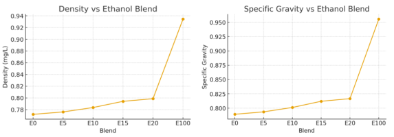
Figure 4. Thermal Analysis of Density and specific.

As illustrated in Figure 4, ethanol density increases from 0.772 mg/L (E0) to 0.9345 mg/L (E100), with specific gravity rising from 0.789 to 0.956. This increase is linked to ethanol’s higher density compared to gasoline, resulting in a greater mass of fuel per unit volume, which may enhance combustion stability. However, gasoline injectors may need recalibration when ethanol levels surpass E20 due to the increased volumetric flow. Ethanol blends from E0 to E20 conform to ASTM D579 specifications, ensuring safety for standard gasoline engines, while E100 requires specialized calibration.

Download: Download full-size image

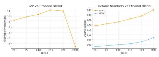
Figure 5. Thermal Analysis RVP, RON, MON and Calorific Value.

In Figure 5, the RVP increases from 9.3 psi (E0) to a peak of 11.2 psi (E15), before dropping sharply to 4.4 psi (E100). The rise up to E15 is attributed to ethanol’s capacity to release lighter hydrocarbons, such as butanes and pentanes, enhancing cold-start performance in low temperatures. The significant drop at higher blends occurs because ethanol has lower volatility, making it less prone to vaporization. Blends E10–E15 are ideal for colder regions, improving cold-start capabilities, while E20–E100 are better suited for hot climates (e.g., Nigeria), as they mitigate vapor lock and reduce evaporative emissions. The RON increases from 119 (E0) to 135 (E100), and the MON rises from 98 to 107. Ethanol's high octane rating contributes to better anti-knock resistance. Higher octane ratings facilitate greater compression ratios, improved combustion timing, and enhanced thermal efficiency, especially under low to medium loads. Additionally, higher ethanol blends (E20+) further improve efficiency in engines designed for high-octane fuels.

Download: Download full-size image

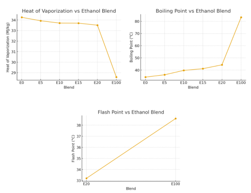
Figure 6. Thermal Analysis; Heat of Vaporization, Flash and Boiling Point.

From Figure 6, the heat of vaporization decreases from 34.25 MJ/kg for E0 to 28.58 MJ/kg for E100. Ethanol’s lower heating value

[9]

implies that a greater mass of fuel is required to deliver the same brake power, which explains the increase in brake-specific fuel consumption (BSFC) observed with higher ethanol blend ratios. Consequently, the energy density of the fuel decreases as ethanol content increases. While ethanol-blended fuels offer notable emission reduction benefits, they generally result in lower fuel economy unless the engine is specifically optimized for ethanol combustion.

The flash point is only noted for higher blends, measuring 33.2°C for E20 and 38.6°C for E100. Increased ethanol content raises the flash point, making the blend safer for storage. While gasoline ignites easily, ethanol makes the mixture less flammable at room temperature. Thus, higher blends (E20–E100) improve storage safety but may hinder cold-start performance in colder climates; however, this is advantageous in warmer regions like Nigeria.

The boiling point also rises with ethanol content, ranging from 34.2°C (E0) to 83.3°C (E100). Ethanol's higher boiling point contributes to lower volatility, slower vaporization, reduced evaporative emissions, and enhanced safety during handling. This can lead to potential cold-start challenges in cooler environments. Therefore, E20–E100 blends are particularly suitable for tropical climates, where ambient warmth offsets the lower volatility.

3.2. Engine Performance

This section presents the effect of ethanol–gasoline blending on engine performance at four load conditions: 3.0 kW, 3.5 kW, 4.0 kW, and 4.5 kW. The key performance parameters evaluated include Brake Thermal Efficiency (BTE), Brake-Specific Fuel Consumption (BSFC), Brake Specific Energy Consumption (BSEC), and Torque Output. The results reflect the influence of ethanol’s physicochemical properties—high octane number, inherent oxygen content, and low heating value on engine combustion behavior.

Table 4. Engine Load 3.0 kW.

PARAMETERS	E0	E5	E10	E15	E20	E100
P Load (kW)	30	30	30	30	30	30
Density ρ (kg/ml)	753	761	767	771	775	792
Time taken t (s)	417	412	404	396	390	386
Fuel volume used per time v (ml)	0.005	0.005	0.005	0.005	0.005	0.005
Speed N (rpm)	2463	2457	2451	2446	2461	2354
Torque T (N)	11.62979	11.65819	11.68673	11.71062	11.63924	12.1683
NT	28644.18	28644.18	28644.18	28644.18	28644.18	28644.18
Heating value Hg (MJ/kg)	34.2525	33.9247	33.7063	33.6992	33.5078	28.5808
Fuel consumption rate MF = v*ρ/t	0.009029	0.009235	0.009493	0.009735	0.009936	0.010259
Fuel equivalent power	0.309258	0.313309	0.31996	0.328057	0.33293	0.293212
Brake power BP	2.003089	2.003089	2.003089	2.003089	2.003089	2.003089
Brake specific fuel consumption BSFC	0.004507	0.004611	0.004739	0.00486	0.00496	0.005122
Brake specific fuel consumption BSEC	0.154391	0.156413	0.159733	0.163775	0.166208	0.14638
Brake thermal efficiency ηbth	6.477077	6.393326	6.260445	6.105926	6.016546	6.831531

In Table 4, E100 demonstrates the highest brake thermal efficiency at 6.83% under the lowest power setting of 3.0 kW, surpassing all intermediate blends, including E0 at 6.48%. Although E100 has a 13.6% higher BSFC (0.00512 kg/kWh compared to 0.004507 kg/kWh), ethanol's superior octane rating and in-cylinder oxygenation enhance combustion completeness, contributing to its 0.35 percentage point advantage. Additionally, E100 achieves a torque of 12.17 Nm, representing a 4.7% increase over E0's 11.63 Nm, maximizing torque output. E20 ranks second among ethanol-gasoline blends for torque at 11.64 Nm and has a thermal efficiency of 6.02%, while E5 and E10 are comparable to E0. The mass fuel flow rate (MF) increases progressively with ethanol content, rising from 0.009205 kg/s (E0) to 0.010039 kg/s (E20) and peaking at 0.010939 kg/s (E100). This 18.8% increase from E0 to E100 is driven by ethanol’s lower heating value (Hg), decreasing from 34.25 MJ/kg (E0) to 28.58 MJ/kg (E100).

Ethanol's higher octane number and oxygenated structure improve both torque output and combustion efficiency. However, due to its lower heating value, more fuel is required to generate the same power, resulting in increased fuel consumption and lower thermal efficiency specifically for brake applications. Torque increments slightly from 11.63 Nm (E0) to 11.64 Nm (E20) and peaks at 12.17 Nm (E100). This 4.6% increase correlates with ethanol's high octane rating (RON ~129 for E20), which mitigates engine knock and allows for advanced ignition timing. Improved knock resistance enhances mechanical efficiency, although these gains are tempered by ethanol’s energy limitations. Engine speed decreases from 2463 rpm (E0) to 2461 rpm (E20) and further to 2354 rpm (E100). The slight increase observed at E20 (2461 rpm compared to 2446 rpm for E15) may indicate experimental variability or transient combustion effects.

Table 5. Engine Load 3.5 kW.

PARAMETERS	E0	E5	E10	E15	E20	E100
P Load (kW)	3.5	3.5	3.5	3.5	3.5	3.5
Density ρ (kg/ml)	753	761	767	771	775	792
Time taken t (s)	412	407	401	393	389	363
Fuel volume used per time v (ml)	0.005	0.005	0.005	0.005	0.005	0.005
Speed N (rpm)	2498	2490	24184	2480	2474	2374
Torque T (N)	13.37798437	13.42097	1.3818312	13.475083	13.50776	14.07675
NT	33418.2049	33418.2	33418.20	33418.20	33418.2	33418.20
Heating value Hg (MJ/kg)	34.2525	33.9247	33.7063	33.6992	33.5078	28.5808
Fuel consumption rate MF = v*ρ/t	0.00913835	0.00934	0.009563	0.009809	0.00996	0.010909
Fuel equivalent power	0.31301131	0.31715	0.322353	0.330560	0.33378	0.311790
Brake power BP	2.33693741	2.33693	2.336937	2.336937	2.33693	2.336937
BSFC	0.00391039	0.004	0.004092	0.004197	0.00426	0.004668
BSEC	0.133940822	0.135715	0.1379383	0.1414505	0.14283	0.133418
Brake thermal efficiency ηbth	7.465983768	7.36836	7.249616	7.0696133	7.001306	7.495215

At a constant brake power of 3.5 kW, Table 5 presents engine performance tests for ethanol-gasoline blends (E0 to E100), revealing trends in energy use, combustion dynamics, and fuel economy. At this power level, E100 again leads the thermal efficiency chart with a notable 7.50%, followed closely by E0 at 7.47%, and significantly ahead of E20 at 7.00%. While E0 reaches a torque peak of 13.38 Nm, E100 exhibits the highest Brake Specific Fuel Consumption (BSFC) at 0.00467 kg/kWh. E15 and E20 follow with thermal efficiencies ranging from 7.07% to 7.00%, illustrating the decline in oxygen content as ethanol's energy content decreases. The mass fuel flow rate (MF) rises progressively with higher ethanol content, increasing from 0.00914 kg/s (E0) to 0.00996 kg/s (E20) and peaking at 0.01091 kg/s (E100). This represents a 19.4% increase from E0 to E100, influenced by ethanol's lower heating value (Hg), which drops from 34.25 MJ/kg (E0) to 28.58 MJ/kg (E100). E100 not only delivers superior engine performance under light to moderate loads but also leverages its knock resistance to optimize combustion phasing at this load. The interaction between improved combustion properties and higher fuel requirements in ethanol-gasoline blends is complex. Torque increases slightly from 13.38 Nm (E0) to 13.51 Nm (E20), peaking at 14.08 Nm (E100). This 5.2% increase corresponds with the high octane rating of ethanol (RON ~129 for E20), which reduces engine knock and facilitates advanced ignition timing. While better knock resistance enhances mechanical efficiency, these benefits are moderated by ethanol’s energy limitations.

Table 6. Engine Load 4.0 kW.

PARAMETERS	E0	E5	E10	E15	E20	E100
P Load (kW)	4.0	4.0	4.0	4.0	4.0	4.0
Density ρ (kg/ml)	753	761	767	771	775	792
Time taken t (s)	409	402	397	390	386	362
Fuel volume used per time v (ml)	0.005	0.005	0.005	0.005	0.005	0.005
Speed N (rpm)	2529	2518	2509	2493	2483	2394
Torque T (N)	15.10171	15.16769	15.22209	15.31979	15.38149	15.95331
NT	38192.23	38192.23	38192.23	38192.23	38192.23	38192.23
Heating value Hg (MJ/kg)	34.2525	33.9247	33.7063	33.6992	33.5078	28.5808
Fuel consumption rate MF = v*ρ/t	0.009205	0.009465	0.00966	0.009885	0.010039	0.010939
Fuel equivalent power	0.315307	0.321103	0.325601	0.333104	0.33638	0.312652
Brake power BP	2.670786	2.670786	2.670786	2.670786	2.670786	2.670786
BSFC	0.003447	0.003544	0.003617	0.003701	0.003759	0.004096
BSEC	0.118058	0.120228	0.121912	0.124721	0.125948	0.117064
Brake thermal efficiency ηbth	8.470423	8.317531	8.202629	8.017882	7.939784	8.542363

In Table 6, at a power setting of 4.0 kW, E100 leads with a brake thermal efficiency (ηᵦth) of 8.54%, compared to 8.47% for E0 and 7.94% for E20. While E100 incurs an 18.8% penalty in Brake Specific Fuel Consumption (BSFC), at 0.004096 kg/kWh versus E0's 0.003447 kg/kWh, it achieves a torque peak of 15.95 Nm, which is 5.6% higher than E0’s 15.10 Nm. E5 and E10 show intermediate efficiencies, ranging from approximately 8.32% to 8.20%, while E20 records the lowest efficiency among the blends. Again, E100 demonstrates the greatest engine performance advantage at this load. The mass fuel flow rate (MF) increases progressively with ethanol content, rising from 0.009205 kg/s (E0) to 0.010039 kg/s (E20) and peaking at 0.010939 kg/s (E100). This represents an 18.8% increase from E0 to E100, driven by ethanol’s lower heating value (Hg), which decreases from 34.25 MJ/kg (E0) to 28.58 MJ/kg (E100). Although ethanol's oxygenated structure enhances combustion completeness, its inherent energy deficit requires higher fuel consumption to sustain the 4.0 kW output. As a result, BSFC rises by 8.9% for E20 (0.003759 kg/kWh) and by 18.8% for E100 (0.004096 kg/kWh), underscoring the energy density penalty associated with ethanol blending.

Brake thermal efficiency (ηbth) drops from 8.47% (E0) to 7.94% (E20), reflecting the combustion inefficiencies linked to ethanol’s lower energy content. However, ηbth marginally rebounds to 8.54% for E100, indicating optimized combustion phasing with pure ethanol due to reduced hydrocarbon interference and stable stoichiometric conditions. This recovery highlights ethanol’s potential for efficient combustion at higher concentrations, assuming engines are recalibrated to utilize its characteristics effectively. Torque increments slightly from 15.10 Nm (E0) to 15.38 Nm (E20) and peaks at 15.95 Nm (E100). This 5.6% increase corresponds with ethanol’s high octane rating (RON ~129 for E20), which mitigates engine knock and allows for advanced ignition timing. Enhanced knock resistance boosts mechanical efficiency, although these gains are somewhat offset by ethanol’s energy limitations. Engine speed decreases from 2529 rpm (E0) to 2483 rpm (E20) and further to 2394 rpm (E100).

Table 7. Engine Load 4.0 kW.

PARAMETERS	E0	E5	E10	E15	E20	E100
P Load (kW)	4.5	4.5	4.5	4.5	4.5	4.5
Density ρ (kg/ml)	753	761	767	771	775	792
Time taken t (s)	406	401	395	386	377	333
Fuel volume used per time v (ml)	0.005	0.005	0.005	0.005	0.005	0.005
Speed N (rpm)	2534	2526	2518	2511	2508	2474
Torque T (N)	16.9559051	17.00961	17.06364	17.11121	17.1316	17.3671
NT	42966.26353	42966.26	42966.26	42966.26	42966.2	42966.2
Heating value Hg (MJ/kg)	34.2525	33.9247	33.7063	33.6992	33.5078	28.5808
Fuel consumption rate MF = v*ρ/t	0.009273399	0.009489	0.0097089	0.009987	0.01027	0.011891
Fuel equivalent power	0.3176371	0.321904	0.3272498	0.336555	0.34441	0.339879
Brake power BP	3.004633813	3.004634	3.0046338	3.004633	3.00463	3.00463
BSFC	0.003086366	0.003158	0.0032313	0.003323	0.00342	0.00395
BSEC	0.105715744	0.107136	0.108915	0.112012	0.11462	0.11311
Brake thermal efficiency ηbth	9.459328949	9.333945	9.1814695	8.927603	8.72399	8.84028

Under the highest load conditions in Table 7, conventional gasoline (E0) regains the lead in thermal efficiency with an ηᵦth of 9.46%, compared to 8.84% for E100. E5 and E10 follow closely with thermal efficiencies of 9.33% and 9.18%, respectively, while E20 drops to 8.72%. Despite this, E100 produces the highest torque at 17.37 Nm, exceeding E0’s 16.96 Nm. This indicates that ethanol’s knock resistance and combustion efficiency continue to enhance peak mechanical output, even though its lower energy density limits overall efficiency. The mass fuel flow rate (MF) steadily increases with the ethanol content, rising from 0.00927 kg/s for E0 to 0.01189 kg/s for E100. This 28% increase in fuel consumption is directly linked to ethanol's lower heating value (Hg), which decreases from 34.25 MJ/kg (E0) to 28.58 MJ/kg (E100). While ethanol's oxygenated molecular structure improves combustion completeness, its inherent energy deficit requires larger fuel volumes to sustain the 4.5 kW output. Consequently, Brake Specific Fuel Consumption (BSFC) rises by 12.8% for E20 (0.00342 kg/kWh) and by 27.8% for E100 (0.00395 kg/kWh), emphasizing the trade-off in energy density. Thermal efficiency (ηbth) decreases from 9.46% (E0) to 8.72% (E20), reflecting the reduced energy content of ethanol. However, there is a slight rebound to 8.84% for E100, suggesting optimized combustion phasing with pure ethanol, likely due to minimized hydrocarbon interference and stable stoichiometric conditions. This underscores the complex relationship between the combustion advantages of ethanol and its energy limitations. Torque experiences a slight increase from 16.96 Nm (E0) to 17.13 Nm (E20), peaking at 17.37 Nm for E100.

Table 8. Engine Performance Ranking at Each Load (E0–E100).

Load (kW)	Best BTE	2nd Best BTE	Worst BTE	Lowest BSFC	Highest Torque	Remarks
3.0 kW	E100 (6.83%)	E0 (6.48%)	E5/E10 (≈6.1%)	E0	E100 (12.17 Nm)	Ethanol’s oxygen improves low-load combustion
3.5 kW	E100 (7.50%)	E0 (7.47%	E20 (7.00%)	E0	E100 (14.08 Nm)	Narrow BTE gap; ethanol still leads
4.0 kW	E100 (8.54%	E0 (8.47%	E20 (7.94%)	E0	E100 (15.95 Nm)	Ethanol maintains efficiency advantage
4.5 kW	E0 (9.46%)	E5/E10	E20 (8.72%)	E0	E100 (17.37 Nm)	Gasoline wins efficiency; ethanol wins torque

Table 9. Overall Performance Across All Loads.

Metric	Best Performer	Reason
Brake Thermal Efficiency (BTE)	E100 (Low–Medium loads	High octane → better timing →more complete combustion
Brake Thermal Efficiency at High Load	E0	Higher heating value → more energy per kg
Brake Specific Fuel Consumption (BSFC)	E0	Highest energy density → lowest fuel mass required
Highest BSFC	E100	Low LHV → more mass needed to maintain power
Torque Output	E100 (All loads)	Faster flame speed & oxygenation → stronger combustion pressure
Best Mid-Blend Performance	E20	Good torque + moderate efficiency + manageable BSFC
Most Efficient for Real-World Climate (Nigeria	E20	Balanced performance + no cold-start issues

Table 10. Blend-by-Blend Overall Rating.

Blend	Efficiency	Fuel Consumption	Torque	Overall Comment
E0 (Gasoline)	High at 4.5 kW	Best (lowest BSFC)	Moderate	Best for high-load efficiency; highest mileage
E5	Slightly improved vs. E0	Slight increase	Slight increase	Minimal difference; safe transitional blend
E10	Similar to E5	Slightly higher BSFC	Slight improvement	Mid-range stability; good general alternative
E15	Moderate	Moderate BSFC	Moderate	Increasing ethanol effect becomes visible
E20	Lower efficiency at high loads	Moderate BSFC	Good torque	Best compromise blend
E100	Best BTE (low–mid loads)	Highest BSFC	Strongest torque at all loads	Requires calibration; best performance, lowest efficiency

3.3. Emission Analysis

This analysis indicates that ethanol-gasoline blends enhance combustion quality due to their oxygenation properties and knock resistance, resulting in lower carbon monoxide (CO) and particulate matter (PM) emissions. However, the trade-offs in nitrogen oxides (NOx) and methane (CH₄) highlight the need for careful selection of blends. The E20 formulation provides a practical compromise, offering environmental advantages while minimizing significant losses in efficiency.

Table 11. Emission Result for 3.0 KW.

GAS	UNIT	E0	E5	E10	E15	E20	E100
O₂	%	15.3	14.8	17.6	17.9	18.2	18.1
CO	Ppm	1.4	1.2	0.99	0.94	0.82	0.62
EFF	%	-	-	-	-	-	-
CO₂	%	0.9	0.8	0.8	0.4	0.4	0.06
NO	Ppm	1.36	1.43	1.51	1.57	1.89	2.33
NO₂	Ppm	0.82	0.78	0.71	0.64	0.62	0.55
NO_X	Ppm	2.18	2.21	2.22	2.21	2.51	2.88
SO2	Ppm	0.87	0.8	0.43	0.12	0.08	0.03
CH₄	%	1.22	1.64	1.91	2.21	2.32	5.52
H₂S	Ppm	2.01	1.14	0.93	0.87	0.72	0.23
VOC	Ppm	8.3	8.5	8.6	8.7	8.9	9.2
PRESSURE	Inwc	–0.02	–0.02	–0.02	–0.02	–0.02	–0.02
LEL	%	Bal	Bal	Bal	Bal	Bal	Bal

As shown in Table 11, the engine's oxygen (O₂, %) concentration begins at 15.3% for E0, slightly decreases to 14.8% at E5, and then rises to 18.1% for E100. This trend indicates that the oxygen levels in the exhaust increase with a higher ethanol percentage. The elevated O₂ levels suggest leaner combustion with some unconsumed oxygen, a characteristic commonly associated with ethanol-blended fuels. Carbon monoxide (CO, ppm) emissions gradually decrease from 1.4 ppm (E0) to 0.62 ppm (E100). This improvement in combustion efficiency due to ethanol results in cleaner burning and reduced CO emissions, highlighting the effectiveness of ethanol blends in lowering carbon monoxide output. Carbon dioxide (CO₂, %) levels drop significantly from 0.9% (E0) to 0.06% (E100). This reduction is due to the lower carbon content of ethanol fuels, suggesting that ethanol combustion is cleaner compared to conventional fuels. Nitric oxide (NO, ppm) concentrations rise from 1.36 ppm (E0) to 2.33 ppm (E100). This increase is likely attributed to the higher combustion temperatures associated with ethanol blends, which tend to enhance NO formation during combustion.

In contrast, nitrogen dioxide (NO₂, ppm) levels decline from 0.82 ppm (E0) to 0.55 ppm (E100). Despite the rising NO levels, the decrease in NO₂ indicates reduced oxidation of NO in the exhaust, potentially linked to the unique combustion chemistry of ethanol. Total nitrogen oxides (NOₓ, ppm) show a slight increase from 2.18 ppm (E0) to 2.88 ppm (E100). This pattern reflects the combined effects of elevated NO levels and reduced NO₂ concentrations, suggesting that nitrogen oxide emissions generally rise with higher ethanol content. Sulfur dioxide (SO₂, ppm) emissions demonstrate a dramatic reduction from 0.87 ppm (E0) to 0.03 ppm (E100), primarily due to ethanol's extremely low sulfur content. Methane (CH₄, %) emissions increase from 1.22% (E0) to 5.52% (E100). This rise suggests that higher ethanol blends may result in additional unburned hydrocarbons, likely due to incomplete combustion at elevated ethanol ratios. Hydrogen sulfide (H₂S, ppm) concentrations decrease from 2.01 ppm (E0) to 0.23 ppm (E100), demonstrating ethanol's effectiveness in reducing emissions of sulfur-containing compounds. Volatile organic compounds (VOC, ppm) show a slight increase from 8.3 ppm (E0) to 9.2 ppm (E100), attributed to the higher volatility of ethanol, which may slightly elevate VOC emissions. Both the lower explosion limit (LEL, %) and pressure (Inwc) remain stable across all blends, recorded at –0.02 Inwc and "Bal." This consistency indicates that the engine operates reliably, with no significant pressure fluctuations or flammability issues observed.

Table 12. Emission Result for 3.5 KW.

GAS	UNIT	E0	E5	E10	E15	E20	E100
O₂	%	14.9	15.4	17.3	17.9	18.2	18.1
CO	Ppm	1.4	1.2	0.99	0.94	0.82	0.62
EFF	%	-	-	-	-	-	-
CO₂	%	0.8	0.6	0.5	0.3	0.1	0.06
NO	Ppm	1.38	1.46	1.54	1.59	1.94	2.45
NO₂	Ppm	0.82	0.78	0.71	0.64	0.62	0.15
NO_X	Ppm	2.2	2.11	1.99	1.96	1.91	0.43
SO2	Ppm	0.87	0.8	0.41	0.1	0.08	0.02
CH₄	%	1.22	1.64	1.91	2.21	2.32	5.52
H₂S	Ppm	2.01	1.14	0.93	0.87	0.72	0.23
VOC	Ppm	8.3	8.4	8.6	8.7	8.7	9.21
PRESSURE	Inwc	–0.02	–0.02	–0.02	–0.02	–0.02	–0.02
LEL	%	Bal	Bal	Bal	Bal	Bal	Bal

Download: Download full-size image

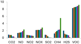
Figure 7. Emission profile at 3.0kW.

The O₂ concentration in Table 12 begins at 14.9% for E0, grows slightly to 15.4% at E5, and then progressively rises to 18.1% for E100. The amount of oxygen in the exhaust increases with a larger ethanol percentage. Because of the oxygen content of ethanol and its different combustion properties, some oxygen is left unconsumed, indicating leaner combustion. The amount of carbon monoxide (CO, ppm) drops from 1.4 ppm (E0) to 0.62 ppm (E100). Ethanol lowers CO emissions by increasing combustion efficiency. This demonstrates the contribution of ethanol blends to cleaner fuel combustion. From 0.8% (E0) to 0.06% (E100), CO₂ decreases. Ethanol fuels produce less CO₂ due to their reduced carbon content. This illustrates how effective ethanol is as a fuel that burns cleanly. Nitric Oxide (NO, ppm) increases to 2.45 ppm (E100) from 1.38 ppm (E0). Higher ethanol blends may cause a modest rise in combustion temperature, which would encourage the generation of NO. This is a common result of faster or hotter combustion.

The concentration of nitrogen dioxide drops from 0.82 ppm (E0) to 0.15 ppm (E100). The decrease in NO₂ indicates reduced NO oxidation in the exhaust at higher ethanol levels, despite the increase in NO. This could be because of changes in exhaust chemistry. There is a noticeable drop in total nitrogen oxides from 2.2 ppm (E0) to 0.43 ppm (E100). In contrast to the 3.0 KW engine, the overall NOₓ emissions decrease with increasing ethanol blends at 3.5 KW, indicating that increased power output may inhibit the generation of total nitrogen oxide. The amount of sulfur dioxide drops dramatically from 0.87 ppm (E0) to 0.02 ppm (E100). Ethanol's advantage in lowering sulfur pollutants is demonstrated by its extremely low sulfur content, which results in significantly lower SO₂ emissions. From 1.22% (E0) to 5.52% (E100), methane (CH₄) increases. Due to incomplete ethanol combustion at high blend ratios, higher ethanol blends produce more unburned hydrocarbons. The concentration of hydrogen sulfide (H2S, ppm) drops from 2.01 ppm (E0) to 0.23 ppm (E100). Because of its low sulfur content, ethanol effectively decreases emissions that contain sulfur. From 8.3 ppm (E0) to 9.21 ppm (E100), there is a modest increase in volatile organic compounds (VOC, ppm). The greater volatility of ethanol, which can marginally increase hydrocarbon emissions, is the cause of the modest rise in VOCs. LEL (%) and pressure (Inwc) are constant for all mixes (–0.02 Inwc and "Bal"). There are no notable variations in pressure or flammability danger during engine running.

Download: Download full-size image

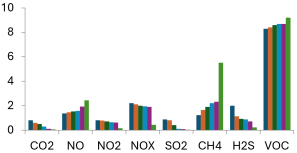
Figure 8. Emission profile at 3.5kW.

Table 13. Emission Result for 4.0 KW.

GAS	UNIT	E0	E5	E10	E15	E20	E100
O2	%	14.9	15.4	17.3	17.9	18.2	18.1
CO	Ppm	1.4	1.2	0.99	0.94	0.82	0.62
EFF	%	-	-	-	-	-	-
CO₂	%	0.8	0.6	0.5	0.3	0.1	0.06
NO	Ppm	1.38	1.46	1.54	1.59	1.94	2.45
NO₂	Ppm	0.82	0.78	0.71	0.64	0.62	0.15
NO_X	Ppm	2.2	2.11	1.99	1.96	1.91	0.43
SO₂	Ppm	0.87	0.8	0.41	0.1	0.08	0.02
CH₄	%	1.22	1.64	1.91	2.21	2.32	5.52
H2S	Ppm	2.01	1.14	0.93	0.87	0.72	0.23
VOC	Ppm	8.3	8.4	8.6	8.6	8.8	8.9
PRESSURE	Inwc	–0.02	–0.02	–0.02	–0.02	–0.02	–0.02
LEL	%	Bal	Bal	Bal	Bal	Bal	Bal

Download: Download full-size image

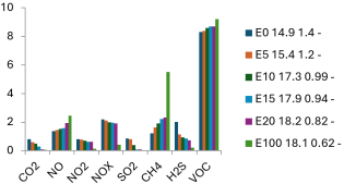
Figure 9. Emission profile at 4.0 kW.

In Table 13, oxygen (O₂,%) grows from 14.9% at E0 to 15.4% at E5 and 18.1% at E100. Because ethanol naturally contains oxygen, a higher ethanol percentage in the fuel results in more unconsumed oxygen in the exhaust, which is a sign of leaner combustion. The amount of carbon monoxide (CO, ppm) drops from 1.4 ppm (E0) to 0.62 ppm (E100). Ethanol increases combustion efficiency, which reduces CO production and produces cleaner exhaust. CO₂(%) decreases from 0.8% (E0) to 0.06% (E100). Ethanol burns cleaner when its carbon concentration is lower because it produces less CO2. Nitric oxide (NO, ppm) rises to 2.45 ppm (E100) from 1.38 ppm (E0). The enhanced local combustion temperatures linked to ethanol mixes are probably the cause of somewhat higher NO generation. The amount of nitrogen dioxide (NO₂, ppm) drops from 0.82 ppm (E0) to 0.15 ppm (E100). NO₂ falls despite increasing NO levels, indicating less NO oxidation in the exhaust with higher ethanol mixes. From 2.2 ppm (E0) to 0.43 ppm (E100), total nitrogen oxides (NOₓ, ppm) decrease. At 3.5 KW, NOₓ generally reduces with ethanol, in contrast to certain lower-power scenarios. This could be because of different combustion kinetics or somewhat lower peak temperatures at higher ethanol percentage. Sulfur Dioxide (SO₂, ppm) decreases to 0.02 ppm (E100) from 0.87 ppm (E0). Because ethanol has relatively little sulfur, SO₂ emissions are drastically reduced. Methane (CH₄,%) increases to 5.52% (E100) from 1.22% (E0). Methane and other unburned hydrocarbons are produced in higher ethanol blends, most likely as a result of incomplete combustion at high ethanol concentrations. From 2.01 ppm (E0) to 0.23 ppm (E100), hydrogen sulfide (H₂S, ppm) drops. Given its low sulfur concentration, ethanol efficiently lowers emissions related to sulfur. Volatile Organic Compounds (VOCs, ppm) show a slight increase from 8.3 ppm (E0) to 8.9 ppm (E100). This minor rise is attributed to the high volatility of ethanol, which can lead to a small increase in hydrocarbon emissions.

Table 14. Emission Result for 4.5 KW.

GAS	UNIT	E0	E5	E10	E15	E20	E100
O₂	%	14.2	14.9	16.9	17.6	18	21.3
CO	ppm	1.4	1.2	0.99	0.94	0.82	0.62
EFF	%	-	-	-	-	-	-
CO₂	%	0.9	0.8	0.8	0.4	0.4	0.06
NO	ppm	1.36	1.43	1.51	1.57	1.89	2.33
NO₂	Ppm	0.82	0.78	0.71	0.64	0.62	0.13
NO_X	Ppm	2.18	2.12	2.1	2.06	2.02	1.98
SO₂	Ppm	0.87	0.8	0.43	0.12	0.08	0.03
CH₄	%	1.22	1.61	1.72	2.21	2.32	5.52
H₂S	Ppm	2.04	1.6	0.95	0.92	0.88	0.23
VOC	Ppm	8.3	8.4	8.6	8.6	8.8	8.9
PRESSURE	Inwc	–0.02	–0.02	–0.02	–0.02	–0.02	–0.02
LEL	%	Bal	Bal	Bal	Bal	Bal	Bal

Oxygen (O₂, %) starts at 14.2% for E0 and gradually increases to 21.3% for E100 in Table 14. Higher ethanol percentages significantly boost O₂ levels in the exhaust, indicating leaner combustion. The more substantial increase observed in higher-powered engines suggests that the oxygen content in ethanol contributes to greater amounts of unused oxygen in the exhaust at elevated loads. The concentration of carbon monoxide (CO, ppm) decreases from 1.4 ppm (E0) to 0.62 ppm (E100). Much like in lower-powered engines, ethanol enhances combustion efficiency, resulting in reduced CO emissions and cleaner exhaust. Carbon dioxide (CO₂, %) drops to 0.06% at E100 after remaining relatively stable for lower blends (0.9–0.8%). The reduced CO₂ levels at higher ethanol blends reflect ethanol's lower carbon content, underscoring its cleaner-burning characteristics. The level of nitric oxide (NO, ppm) increases from 1.36 ppm (E0) to 2.33 ppm (E100). Despite the modest rise at higher power, the elevated NO levels suggest that ethanol may contribute to increased local combustion temperatures, thereby enhancing NO production. Nitrogen dioxide (NO₂, ppm) experiences a decrease from 0.82 ppm (E0) to 0.13 ppm (E100). As ethanol concentration in the exhaust rises, the decline in NO₂ occurs despite the increase in NO, indicating reduced NO oxidation. Total nitrogen oxides (NOₓ, ppm) show a slight decrease from 2.18 ppm (E0) to 1.98 ppm (E100). In engines operating at 4.5 kW, total NOₓ emissions decrease slightly with higher ethanol blends, unlike in lower-power engines. This could be attributed to more rapid exhaust dilution or lower peak combustion temperatures. From 0.87 ppm (E0) to 0.03 ppm (E100), sulfur dioxide (SO₂, ppm) decreases dramatically. Since ethanol has virtually little sulfur, SO₂ emissions are significantly reduced. Methane (CH₄,%) rises to 5.52% (E100) from 1.22% (E0). Incomplete combustion at high ethanol ratios is consistent with higher ethanol blends producing more unburned hydrocarbons. From 2.04 ppm (E0) to 0.23 ppm (E100), hydrogen sulfide (H₂S, ppm) decreases. Ethanol's environmental benefit is confirmed by its effective reduction of emissions containing sulfur. There is a little rise in volatile organic compounds (VOC, ppm) from 8.3 ppm (E0) to 8.9 ppm (E100). The higher volatility of ethanol can lead to a modest increase in VOC emissions.

Download: Download full-size image

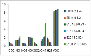
Figure 10. Emission profile at 4.5 kW.

3.3.1. Particulate Matter (PM)

Ethanol’s sulphur-free nature and inherent oxygen content substantially reduce particulate matter (PM) precursors. Sulphur dioxide (SO₂) a critical driver of PM nucleation decreased sharply with increasing ethanol content, falling by 91% in E20 (0.08 ppm) and by 98% in E100 (0.02 ppm) relative to E0 (0.87 ppm). The presence of oxygen in ethanol promotes more complete oxidation of carbon-rich zones in fuel-rich combustion regions, thereby suppressing soot formation

[17]

. Although direct PM measurements were not conducted in this study, the pronounced reduction in SO₂ strongly indicates a corresponding decrease in PM emissions, given the dominant role of sulphur-induced nucleation in gasoline engine particulate formation. Future investigations incorporating gravimetric filter analysis or scanning electron microscopy (SEM) are recommended to directly quantify and characterize PM emissions and to validate these findings.

3.3.2. Nitrogen Oxides (NOx)

NOx emissions exhibited a dual trend: total NOx decreased by 13% for E20 (1.91 ppm) and 80% for E100 (0.43 ppm), but nitric oxide (NO) a potent smog precursor increased by 39% (E20) and 78% (E100). This divergence stems from ethanol’s high adiabatic flame temperature, which accelerates thermal NO formation via the Zeldovich mechanism. Concurrently, ethanol-derived hydroxyl radicals quench nitrogen dioxide (NO₂), reducing its concentration by 24% (E20) and 82% (E100). For E100, total NOx (0.43 ppm) complies with Euro 6 standards (≤0.08 g/kWh), but E20 (1.91 ppm) exceeds thresholds, necessitating aftertreatment systems like exhaust gas recirculation (EGR) or selective catalytic reduction (SCR).

3.3.3. Carbon Monoxide (CO)

CO emissions decreased steadily with ethanol content, falling by 41% for E20 (0.82 ppm) and 56% for E100 (0.62 ppm). This reduction, which is driven by ethanol's oxygen-enriched combustion, is consistent with 30-50% CO reductions in E10-E30 mixes

[15]

. Higher exhaust oxygen levels (14.9% for E0 to 18.2% for E20) indicate improved CO-to-CO₂ oxidation, supporting ethanol's function in improving urban air quality. All blends comfortably met Euro 6 CO limits (≤1.0 g/kWh), underscoring ethanol’s viability as a transitional fuel.

3.3.4. Unburned Hydrocarbons (HC)

Methane (CH₄) and volatile organic compounds (VOCs), which are indicators of HC emissions, rose dramatically as the amount of ethanol increased. The high latent heat of vaporization of ethanol, which cools combustion chambers and encourages partial oxidation, is responsible for the 353% increase in CH₄ for E100 (5.52%). HC decreases which is attributed to variations in ethanol purity or combustion phasing. The climatic impact of CH₄ may be overlooked by regulatory systems that focus on total HC (such as Euro 6), since methane has a 28–36 times greater potential for global warming over a 100-year period than CO₂.

The inferred reduction in particulate matter (PM) emissions is consistent with literature indicating that oxygenated fuels suppress soot formation by promoting oxidation of carbon-rich zones during fuel-rich combustion

[16]

. Nonetheless, the absence of direct PM measurements in this study limits the certainty of emission-control policy implications

[17]

. Furthermore, the pronounced increase in methane (CH₄) emissions, observed alongside high ethanol blends, is attributed to ethanol’s charge-cooling effect, which lowers in-cylinder temperatures and favors partial oxidation pathways. By quantifying methane’s contribution to total hydrocarbon emissions, this study extends current understanding of ethanol–gasoline blends’ impact on both local air quality and climate-relevant pollutants.

The efficiency and emission trends observed in this study both corroborate and diverge from findings reported in previous research. The increase in NO emissions observed for E20–E100 contrasts with some earlier studies, which reported minimal NOₓ formation at moderate ethanol blending ratios

[13, 14]

. This discrepancy may be attributable to differences in combustion temperature, in-cylinder pressure, and engine calibration, highlighting the critical role of engine design in modulating the thermal NOₓ pathway. Similarly, the measured increase in brake-specific fuel consumption (BSFC) of 10–28% aligns with prior reports

[13]

, reflecting ethanol’s lower lower heating value (LHV) compared with conventional gasoline. However, the torque recovery observed at E100 departs from the generally reported trend of progressive torque reduction with increasing ethanol content

[14, 15]

. This suggests that engine-specific optimization, such as ignition timing adjustment and fuel injection calibration, can mitigate high-ethanol torque penalties. Overall, the findings emphasize the interplay between fuel properties, engine design, and calibration, providing insights for optimizing ethanol blend ratios to balance efficiency, torque performance, and emission reduction.

4. Conclusion

This study confirms the technical viability of palm-sap ethanol as a renewable blending component for gasoline engines and demonstrates its capacity to reduce vehicular emissions while enhancing engine performance. Ethanol–gasoline blends, particularly E15 and E20, present effective options for mitigating urban air pollution, improving engine torque, and promoting the utilization of locally available renewable resources.

Overall, the findings support the adoption of E20 as a transitional transportation fuel capable of contributing to Nigeria’s low-carbon energy goals without compromising engine compatibility or performance. Higher blend ratios lead to higher fuel consumption and methane emissions, but when appropriate calibration and aftertreatment systems are used, the performance and environmental advantages greatly exceed these disadvantages. In addition to supporting ethanol's position in Nigeria's low-carbon energy transition, this study offers useful information for more general policy, technical, and scholarly discussions.

Abbreviations

Mf	Fuel Consumption Rate (kg/s)
V	Volume of Fuel Used per Time (m3)
ρ	Density of Fuel (kg/m3)
t	Time Taken (s)
Pf	Fuel Equivalent Power (W)
Hg	Heating Value (MJ/kg)
BP	Brake Power (kW)
N	Speed (rpm)
T	Torque (N m)
BSFC	Brake Specific Fuel Consumption (kg/kWh)
BSEC	Brake Specific Energy Consumption (kJ/kWh)
ηbth	Brake Thermal Efficiency (%)
AFR	Air-Fuel Ratio
RON	Research Octane Number
ASTM	American Society for Testing and Material
PM	Particulate Matter
RVP	Reid Vapour Pressure
LHV	Lower Heat of Vapourization
ECU	Electronic Cntrol Unit
O₂	Oxygen
CO	Carbon Monoxide
EEF	Emission Enhancement Factor
CO₂	Carbon Dioxide
NO	Nitric Oxide
NO₂	Nitrogen Dioxide
NO_X	Oxides of Nitrogen
SO₂	Sulfur Dioxide
CH₄	Methane
VOC	Volatile Organic Componds
LEL	Lower Explosive Limit

Author Contributions

Shehu Sule Aboje: Data curation, Resource, investigation, methodology

Toyin Olabisi Odutola: Conceptualization, formal analysis

Funding

The authors did not receive funding from any organization.

Conflicts of Interest

The authors declare no conflicts of interest.

References

[1]	Kawaguchi, S., Takahashi, K., & Satoh, K. (2021). Electron collision cross section set for N₂ and electron transport in N₂, N₂/He, and N₂/Ar. Plasma Sources Science and Technology, 30(3), 035010.
[2]	Wilberforce, T., Olabi, A. G., Sayed, E. T., Elsaid, K., & Abdelkareem, M. A. (2021). Progress in carbon capture technologies. Science of The Total Environment, 761, 143203.
[3]	Rose, C. (2022). Enforcing the ‘community interest’in combating transnational crimes: the potential for public interest litigation. Netherlands International Law Review, 69(1), 57-82.
[4]	Gbakon, K. 2020. To What Extent does Nigeria's Biofuel Policy offer Fiscal Incentives.
[5]	Liu, S., Lin, Z., Zhang, H., Fan, Q., Lei, N., & Wang, Z. (2023). Experimental study on combustion and emission characteristics of ethanol-gasoline blends in a high compression ratio SI engine. Energy, 274, 127398.
[6]	Anish Raman, C., Varatharajan, K., Abinesh, P. & Venkatachalapathi, N. “Analysis of MTBE as an oxygenate additive to gasoline,” International Journal of Engineering Research and Applications, vol. 4, Issue 3, pp. 712-718, 2021.
[7]	Oral, F. (2024). Effect of using gasoline and gasoline-ethanol fuel mixture on performance and emissions in a hydrogen generator supported SI engine. Case Studies in Thermal Engineering, 55, 104192.
[8]	Han, J., He, W., & Somers, L. M. T. (2020). Experimental investigation of performance and emissions of ethanol and n-butanol fuel blends in a heavy-duty diesel engine. Frontiers in Mechanical Engineering, 6, 26.
[9]	Mohammed, Mortadha. K. & Balla, Hyder & Al Dulaimi, Zaid & S. kareem, Zaid & Al-Zuhairy, Mudhaffar. (2021). Effect of Ethanol-Gasoline Blends on SI Engine Performance and Emissions. Case Studies in Thermal Engineering. 25. 100891. https://doi.org/10.1016/j.csite.2021.100891
[10]	Ruwe, L., Cai, L., Wullenkord, J., Schmitt, S. C., Felsmann, D., Baroncelli, M.,... & Kohse-Höinghaus, K. (2021). Low-and high-temperature study of n-heptane combustion chemistry. Proceedings of the Combustion Institute, 38(1), 405-413.
[11]	Song, T., Wang, C., Wen, M., Liu, H., & Yao, M. (2024). Combustion mechanism study of ammonia/n-dodecane/n-heptane/EHN blended fuel. Applications in Energy and Combustion Science, 17, 100241.
[12]	Wen, M., Liu, H., Cui, Y., Ming, Z., Feng, L., Wang, G., & Yao, M. (2023). Study on combustion stability and flame development of ammonia/n-heptane dual fuel using multiple optical diagnostics and chemical kinetic analyses. Journal of Cleaner Production, 428, 139412.
[13]	Najafi, B. Ghobadian, T. Tavakoli, D. R. Buttsworth, T. F. Yusaf, M. Faizollahnejad, Performance and exhaust emissions of a gasoline engine with ethanol blended gasoline fuels using artificial neural network, Applied Energy, Volume 86, Issue 5, 2009, Pages 630-639, https://doi.org/10.1016/j.apenergy.2008.09.017
[14]	Costa, R. C., Ramos, M. D. N., Fleck, L., Gomes, S. D., & Aguiar, A. (2020). Critical analysis and predictive models using the physicochemical characteristics of cassava processing wastewater generated in Brazil. Journal of Water Process Engineering, 47, 102629.
[15]	Agarwal, A. K. et al. (2019). CO reduction in ethanol-gasoline blends. Fuel Processing Technology.
[16]	Heywood, J. B. (2018). Internal Combustion Engine Fundamentals. McGraw-Hill.
[17]	Zhu, L. et al. (2019). PM reduction in oxygenated fuels. Environmental Science & Technology.

Cite This Article

Plain Text BibTeX RIS

APA Style

Aboje, S. S., Odutola, T. O. (2026). Combustible Ethanol-Gasoline Blend for Reduced Carbon Monoxide Emission. Petroleum Science and Engineering, 10(1), 17-36. https://doi.org/10.11648/j.pse.20261001.12

Copy | Download

ACS Style

Aboje, S. S.; Odutola, T. O. Combustible Ethanol-Gasoline Blend for Reduced Carbon Monoxide Emission. Pet. Sci. Eng. 2026, 10(1), 17-36. doi: 10.11648/j.pse.20261001.12

Copy | Download

AMA Style

Aboje SS, Odutola TO. Combustible Ethanol-Gasoline Blend for Reduced Carbon Monoxide Emission. Pet Sci Eng. 2026;10(1):17-36. doi: 10.11648/j.pse.20261001.12

Copy | Download

@article{10.11648/j.pse.20261001.12,
  author = {Shehu Sule Aboje and Toyin Olabisi Odutola},
  title = {Combustible Ethanol-Gasoline Blend for Reduced Carbon Monoxide Emission},
  journal = {Petroleum Science and Engineering},
  volume = {10},
  number = {1},
  pages = {17-36},
  doi = {10.11648/j.pse.20261001.12},
  url = {https://doi.org/10.11648/j.pse.20261001.12},
  eprint = {https://article.sciencepublishinggroup.com/pdf/10.11648.j.pse.20261001.12},
  abstract = {This study presents the emission profiles and combustion characteristics of ethanol-gasoline blends in internal combustion engines with the goal of reducing environmental impact and increasing efficiency in Nigeria. The goal of the project is to assess the exhaust emissions and combustion properties of different ethanol-gasoline blends in internal combustion engines to increase efficiency and lessen environmental effect. Palm sap was used to make ethanol, which was then combined with gasoline from the Dangote Refinery's MRS filling station to create mixes E5 (95% gasoline), E10 (90% gasoline), E15 (85% gasoline), and E20 (80% gasoline). To establish performance criteria for these blends, known concentrations of n-heptane were added. The following physicochemical investigations were performed: density and specific gravity, octane rating, flash point, boiling point range, Reid Vapor Pressure (RVP), and heating value. In addition, engine performance was measured at different engine torque levels (3.0, 3.5, 4.0, and 4.5 kW) to compute the corresponding speed, brake specific energy consumption (BSEC), brake specific fuel consumption (BSFC), fuel equivalent power (FEP), and brake thermal efficiency (BTE). Emission tests were also conducted to evaluate gas emissions in compliance with environmental standards and regulations. Blends of ethanol and gasoline, particularly E15 and E20, provide promising ways to reduce air pollution in cities, boost engine torque, and use renewable resources that are harvested locally. In addition to providing helpful information for more general policy, technical, and scholarly conversations, this study highlights the role that ethanol plays in Nigeria's low-carbon energy transition.},
 year = {2026}
}

Copy | Download

TY  - JOUR
T1  - Combustible Ethanol-Gasoline Blend for Reduced Carbon Monoxide Emission
AU  - Shehu Sule Aboje
AU  - Toyin Olabisi Odutola
Y1  - 2026/02/27
PY  - 2026
N1  - https://doi.org/10.11648/j.pse.20261001.12
DO  - 10.11648/j.pse.20261001.12
T2  - Petroleum Science and Engineering
JF  - Petroleum Science and Engineering
JO  - Petroleum Science and Engineering
SP  - 17
EP  - 36
PB  - Science Publishing Group
SN  - 2640-4516
UR  - https://doi.org/10.11648/j.pse.20261001.12
AB  - This study presents the emission profiles and combustion characteristics of ethanol-gasoline blends in internal combustion engines with the goal of reducing environmental impact and increasing efficiency in Nigeria. The goal of the project is to assess the exhaust emissions and combustion properties of different ethanol-gasoline blends in internal combustion engines to increase efficiency and lessen environmental effect. Palm sap was used to make ethanol, which was then combined with gasoline from the Dangote Refinery's MRS filling station to create mixes E5 (95% gasoline), E10 (90% gasoline), E15 (85% gasoline), and E20 (80% gasoline). To establish performance criteria for these blends, known concentrations of n-heptane were added. The following physicochemical investigations were performed: density and specific gravity, octane rating, flash point, boiling point range, Reid Vapor Pressure (RVP), and heating value. In addition, engine performance was measured at different engine torque levels (3.0, 3.5, 4.0, and 4.5 kW) to compute the corresponding speed, brake specific energy consumption (BSEC), brake specific fuel consumption (BSFC), fuel equivalent power (FEP), and brake thermal efficiency (BTE). Emission tests were also conducted to evaluate gas emissions in compliance with environmental standards and regulations. Blends of ethanol and gasoline, particularly E15 and E20, provide promising ways to reduce air pollution in cities, boost engine torque, and use renewable resources that are harvested locally. In addition to providing helpful information for more general policy, technical, and scholarly conversations, this study highlights the role that ethanol plays in Nigeria's low-carbon energy transition.
VL  - 10
IS  - 1
ER  -

Copy | Download

Author Information

Shehu Sule Aboje

Mechatronics and Automation Department, Industrial Training Fund-MSTC, Abuja, Nigeria

http://orcid.org/0009-0005-1042-1778
Toyin Olabisi Odutola

Department of Petroleum and Gas Engineering, University of Port Harcourt, Port Harcourt, Nigeria

Contact Email

http://orcid.org/0000-0002-9996-5392

Download PDF

Submit an Article

Plain Text BibTeX RIS

APA Style

Aboje, S. S., Odutola, T. O. (2026). Combustible Ethanol-Gasoline Blend for Reduced Carbon Monoxide Emission. Petroleum Science and Engineering, 10(1), 17-36. https://doi.org/10.11648/j.pse.20261001.12

Copy | Download

ACS Style

Aboje, S. S.; Odutola, T. O. Combustible Ethanol-Gasoline Blend for Reduced Carbon Monoxide Emission. Pet. Sci. Eng. 2026, 10(1), 17-36. doi: 10.11648/j.pse.20261001.12

Copy | Download

AMA Style

Aboje SS, Odutola TO. Combustible Ethanol-Gasoline Blend for Reduced Carbon Monoxide Emission. Pet Sci Eng. 2026;10(1):17-36. doi: 10.11648/j.pse.20261001.12

Copy | Download

@article{10.11648/j.pse.20261001.12,
  author = {Shehu Sule Aboje and Toyin Olabisi Odutola},
  title = {Combustible Ethanol-Gasoline Blend for Reduced Carbon Monoxide Emission},
  journal = {Petroleum Science and Engineering},
  volume = {10},
  number = {1},
  pages = {17-36},
  doi = {10.11648/j.pse.20261001.12},
  url = {https://doi.org/10.11648/j.pse.20261001.12},
  eprint = {https://article.sciencepublishinggroup.com/pdf/10.11648.j.pse.20261001.12},
  abstract = {This study presents the emission profiles and combustion characteristics of ethanol-gasoline blends in internal combustion engines with the goal of reducing environmental impact and increasing efficiency in Nigeria. The goal of the project is to assess the exhaust emissions and combustion properties of different ethanol-gasoline blends in internal combustion engines to increase efficiency and lessen environmental effect. Palm sap was used to make ethanol, which was then combined with gasoline from the Dangote Refinery's MRS filling station to create mixes E5 (95% gasoline), E10 (90% gasoline), E15 (85% gasoline), and E20 (80% gasoline). To establish performance criteria for these blends, known concentrations of n-heptane were added. The following physicochemical investigations were performed: density and specific gravity, octane rating, flash point, boiling point range, Reid Vapor Pressure (RVP), and heating value. In addition, engine performance was measured at different engine torque levels (3.0, 3.5, 4.0, and 4.5 kW) to compute the corresponding speed, brake specific energy consumption (BSEC), brake specific fuel consumption (BSFC), fuel equivalent power (FEP), and brake thermal efficiency (BTE). Emission tests were also conducted to evaluate gas emissions in compliance with environmental standards and regulations. Blends of ethanol and gasoline, particularly E15 and E20, provide promising ways to reduce air pollution in cities, boost engine torque, and use renewable resources that are harvested locally. In addition to providing helpful information for more general policy, technical, and scholarly conversations, this study highlights the role that ethanol plays in Nigeria's low-carbon energy transition.},
 year = {2026}
}

Copy | Download

TY  - JOUR
T1  - Combustible Ethanol-Gasoline Blend for Reduced Carbon Monoxide Emission
AU  - Shehu Sule Aboje
AU  - Toyin Olabisi Odutola
Y1  - 2026/02/27
PY  - 2026
N1  - https://doi.org/10.11648/j.pse.20261001.12
DO  - 10.11648/j.pse.20261001.12
T2  - Petroleum Science and Engineering
JF  - Petroleum Science and Engineering
JO  - Petroleum Science and Engineering
SP  - 17
EP  - 36
PB  - Science Publishing Group
SN  - 2640-4516
UR  - https://doi.org/10.11648/j.pse.20261001.12
AB  - This study presents the emission profiles and combustion characteristics of ethanol-gasoline blends in internal combustion engines with the goal of reducing environmental impact and increasing efficiency in Nigeria. The goal of the project is to assess the exhaust emissions and combustion properties of different ethanol-gasoline blends in internal combustion engines to increase efficiency and lessen environmental effect. Palm sap was used to make ethanol, which was then combined with gasoline from the Dangote Refinery's MRS filling station to create mixes E5 (95% gasoline), E10 (90% gasoline), E15 (85% gasoline), and E20 (80% gasoline). To establish performance criteria for these blends, known concentrations of n-heptane were added. The following physicochemical investigations were performed: density and specific gravity, octane rating, flash point, boiling point range, Reid Vapor Pressure (RVP), and heating value. In addition, engine performance was measured at different engine torque levels (3.0, 3.5, 4.0, and 4.5 kW) to compute the corresponding speed, brake specific energy consumption (BSEC), brake specific fuel consumption (BSFC), fuel equivalent power (FEP), and brake thermal efficiency (BTE). Emission tests were also conducted to evaluate gas emissions in compliance with environmental standards and regulations. Blends of ethanol and gasoline, particularly E15 and E20, provide promising ways to reduce air pollution in cities, boost engine torque, and use renewable resources that are harvested locally. In addition to providing helpful information for more general policy, technical, and scholarly conversations, this study highlights the role that ethanol plays in Nigeria's low-carbon energy transition.
VL  - 10
IS  - 1
ER  -

Copy | Download