A Weighted Ensemble Learning Approach with Synthetic Oversampling for Maize Yield Modeling in Data-limited Agro-ecological Zones of Uganda

Danison Taremwa; Emmanuel Ahishakiye; Aggrey Obbo; Paul Kategaya Kisozi; Fred Kaggwa

doi:doi:10.11648/j.ajai.20261001.21

Research Article |

| Peer-Reviewed

A Weighted Ensemble Learning Approach with Synthetic Oversampling for Maize Yield Modeling in Data-limited Agro-ecological Zones of Uganda

Danison Taremwa^*

, Emmanuel Ahishakiye

, Aggrey Obbo

, Paul Kategaya Kisozi

, Fred Kaggwa

Published in American Journal of Artificial Intelligence (Volume 10, Issue 1)

Received: 1 February 2026 Accepted: 14 February 2026 Published: 27 February 2026

Views: Downloads:

Download PDF

Share This Article

Twitter
Linked In
Facebook

Abstract

Sparse and irregular agricultural records constrain reliable crop yield modelling in many Sub-Saharan African regions. This study evaluates the use of ensemble machine learning combined with synthetic oversampling for maize yield modelling in data-limited agro-ecological zones of Uganda. Seasonal climatic variables, including rainfall, soil moisture, temperature, and solar radiation, were aggregated from satellite-derived datasets and integrated with maize-yield records from the Uganda Bureau of Statistics for 2018–2020. To address severe data imbalance and scarcity, the Synthetic Minority Oversampling Technique for Regression with Gaussian Noise (SMOGN) was employed to enhance representation of low- and high-yield conditions. An ensemble model combining LightGBM, Random Forest, and Decision Tree algorithms was developed and compared with individual machine-learning and deep-learning models. The ensemble achieved a coefficient of determination of approximately 0.99 and a root-mean-square error of approximately 0.06 t/ha, outperforming individual tree-based models and deep learning baselines (R² ≈ 0.79–0.83). Feature importance analysis indicated that soil moisture, rainfall, and solar radiation were the dominant climatic drivers of yield variability across zones. However, because a substantial proportion of the training samples were synthetically generated and the observations span only three years, the model should be interpreted as a methodological demonstration rather than as an operational yield-forecasting system. The findings indicate that combining ensemble learning with controlled synthetic data augmentation can support agricultural modelling in environments where long-term yield measurements are scarce. The proposed approach provides a foundation for future work incorporating extended field observations and independent validation datasets.

Published in	American Journal of Artificial Intelligence (Volume 10, Issue 1)
DOI	10.11648/j.ajai.20261001.21
Page(s)	114-135
Creative Commons	This is an Open Access article, distributed under the terms of the Creative Commons Attribution 4.0 International License (http://creativecommons.org/licenses/by/4.0/), which permits unrestricted use, distribution and reproduction in any medium or format, provided the original work is properly cited.
Copyright	Copyright © The Author(s), 2026. Published by Science Publishing Group

Keywords

Crop Yield Prediction, Ensemble Learning, Meteorological Data, SMOGN (Synthetic Oversampling), Precision Agriculture

1. Introduction

Maize, a vital global food crop, plays a crucial role in ensuring food security and human survival, particularly in Africa and Latin America, where it is essential for low-income populations

[1]

. Cultivated on 200 million hectares annually, it yields over a billion tonnes, making it one of the most widely grown crops globally

[2]

. Over the past 25 years, global maize production has more than doubled, due to genetic improvements (+50%) and expanded cultivation areas (+46%)

[3]

. Yet, yield gains in Sub-Saharan Africa (SSA) have lagged significantly behind those in Asia and the Americas

[4]

. For instance, Uganda's maize yield is about 2.5 tonnes per hectare (t/ha), which is barely half the global average (5–7 t/ha) and one-quarter of the United States’ yields, and is projected to decline by approximately 10% between 2021 and 2040

[5]

. This deficit is exacerbated by the fact that up to 40% of cereal production land is experiencing yield stagnation, due to climatic stress, soil degradation, and biophysical constraints

[6, 7]

. As a result, hunger in SSA is resurging after years of decline, marking a significant reversal of the global trend toward declining food insecurity

[8]

. These trends jeopardize the achievements of “Zero Hunger” (United Nations Sustainable Development Goal 2) in Africa, underscoring the need for more effective agricultural management strategies

[9, 10]

Therefore, precise measurement of food insecurity is crucial for assessing the extent of the issue and developing effective policies and programs to mitigate it. A fundamental component of food insecurity evaluation is the accurate quantification of crop yields, which helps estimate food availability and overall productive capacity

[11]

,. For instance, the seasonal estimation of large-scale maize yields can enhance the assessment of environmental stress responses, providing reliable information to support sustainable adaptations in agricultural cropping systems

[12]

. As a result, accurate maize yield statistics, particularly during critical stages of the growing season, enable farmers to make timely and informed decisions regarding resource management, including fertilizer application, irrigation planning, and pest control

[13]

. This helps agricultural stakeholders prepare for potential hazards, thereby preventing yield loss, reducing costs, and boosting productivity to achieve optimal results

[14]

However, predicting crop yield is one of the most complex challenges in precision agriculture, and numerous models have been developed and validated for this purpose

[15]

. This challenge requires the use of multiple features, as agricultural output depends on various parameters, including soil, fertilizer use, climate, weather, seed variety, and interactions that occur during plant development

[16, 17]

. This underscores that predicting crop yield is a multiphase, data-intensive process, in which achieving greater accuracy at large spatial scales is essential to minimize financial losses and support effective agricultural planning and policymaking

[18]

1.1. Motivation of the Study

Maize is central to Uganda’s food system and rural incomes. Sector evidence indicates that maize is grown on more than 1.9 million hectares, accounting for about 20% of the country’s total crop area; therefore, production shocks can quickly affect food availability, animal-feed costs, and cross-border markets within the East African Community

[19]

. Timely, quantitative pre-harvest yield estimates therefore matter for input planning, storage, pricing, and food-security preparedness, supporting extension and market decisions. Historically, maize yield prediction (MYP) in Uganda relied on field-based methods, including farmer surveys, manual sampling, and empirical agronomic models

[20]

. Yields are then predicted using regression equations applied to field samples, assuming the samples represent uniform conditions (e.g., consistent soil nutrient levels and water availability), and extrapolating these relationships to whole fields

[21]

. These methods are interpretable and can perform well with limited features; however, expert judgement, sampling design, and self-reported data can significantly influence the accuracy of these estimates

[22]

. For example,

[23]

employed ground-based measurements and regression modelling to predict maize yields in Eastern Uganda, achieving an R-squared value of 0.54. Moreover, implementing this approach across large, geographically remote areas is often resource-intensive and time-consuming. This can result in significant delays in providing maize yield estimates to farmers and policymakers, thereby reducing their ability to make timely decisions that enhance productivity and minimize yield losses

[24]

. These challenges highlight the urgent need for innovative, data-driven yield prediction methods that can scale and deliver more granular, timely forecasts.

The increasing availability of Earth observation (EO) data enables repeated monitoring of vegetation and environmental conditions over large areas. Reviews of heterogeneous African maize systems argue that improvements in sensors and open-access products are making EO-assisted yield estimation increasingly feasible

[16]

. However, broader research on satellite imagery with machine learning cautions that when ground data are scarce or noisy, models can overfit and reported skill can be exaggerated by weak validation designs

[25]

. In this study, maize yields (from the Uganda Bureau of Statistics (UBOS)) are available only for 2018–2020 and are reported biannually (two seasons per year) across ten ZARDI zones, yielding 60 season–zone observations

[26]

. Such small samples create predictable modelling risks: unstable estimates of climate–yield relationships, high sensitivity to how data are split for training and testing, and difficulty learning rare low- and high-yield seasons

[27]

The research gap is, therefore, methodological. Uganda lacks evidence on how to produce quantitative, ZARDI-specific pre-harvest maize yield forecasts that remain stable under extreme label scarcity and yield imbalance. This study addresses a focused methodological question: under severe data scarcity and yield imbalance, can an ensemble of powerful tabular-data learners, combined with controlled synthetic data augmentation, improve modelling stability and predictive consistency? Benchmark evidence on tabular prediction suggests that tree ensembles often outperform deep learning alternatives and require less extensive tuning, an advantage when samples are small. SMOGN (Synthetic Minority Over-sampling Technique for Regression with Gaussian Noise) addresses imbalanced regression by generating synthetic samples in under-represented target ranges, improving representation of extreme outcomes without changing the intent of the original target variable

[28]

. Accordingly, the study integrates aggregated climatic predictors, rainfall, temperature, solar radiation, and soil-moisture proxies from open EO and reanalysis services, aligning daily inputs with seasonal yield reporting. SMOGN expands the modelling dataset from 60 to 295 records, after which a weighted ensemble combining LightGBM, Random Forest, and Decision Tree learners is trained with weights derived from validation errors. Because most training instances are synthetic and the real observations span only three years, the study does not claim to have an operational forecasting system. Rather, it is to provide a transparent proof of concept that demonstrates how weighted ensemble and imbalanced-regression augmentation can be designed and interpreted in data-limited agro-ecological zones, and what additional real-yield data and independent validation would be needed before deployment under typical Sub-Saharan African constraints.

This study, therefore, aims to investigate whether combining ensemble machine learning methods with controlled synthetic data augmentation can support maize yield modelling under severe agricultural data scarcity. Specifically, the study seeks to:

i. Integrate multi-source climatic variables, including rainfall, soil moisture, solar radiation, and temperature, with limited historical maize yield records across Uganda’s ZARDI agro-ecological zones.

ii. Apply SMOGN-based synthetic oversampling to mitigate yield imbalance and sparse observations while aiming to preserve the statistical characteristics of the original dataset.

iii. Develop and experimentally evaluate an ensemble modelling approach combining LightGBM, Random Forest, and Decision Tree algorithms using a short temporal dataset (2018–2020; 60 season–zone observations).

iv. Analyze the relative importance of different climatic variables in explaining maize yield variability across the heterogeneous agro-ecological zones.

1.2. Contributions of the Study

Rather than presenting an operational yield-forecasting system, this work provides a methodological investigation of machine learning under the real-world data limitations typical of many Sub-Saharan African agricultural contexts. The main contributions are:

i. Demonstrates the feasibility of ensemble learning for crop yield modelling using extremely limited agricultural records.

ii. Provides an experimental evaluation of SMOGN-based synthetic oversampling for regression problems in agricultural datasets characterized by imbalance and small sample size.

iii. Identifies dominant climatic predictors of maize yield variability, particularly soil moisture, rainfall, and solar radiation, across heterogeneous agro-ecological zones.

iv. Offers a reproducible modelling framework that can be extended and externally validated when longer-term yield observations become available.

The study, therefore, serves as a proof-of-concept methodological framework for applying machine learning in regions where consistent long-term agricultural measurements are scarce, rather than a deployment-ready forecasting tool.

1.3. Paper Organization

The remainder of this paper is structured as follows. Section 2 reviews related literature on machine learning approaches for crop yield modelling and discusses previous studies on ensemble learning and data augmentation techniques. Section 3 describes the study area, datasets, preprocessing procedures, SMOGN-based synthetic oversampling, and the proposed ensemble modelling framework. Section 4 presents the experimental setup and performance evaluation of the individual models and the ensemble approach. Section 5 discusses the results, interprets the influence of climatic variables, and examines the implications and limitations of modelling under data scarcity. Finally, Section 6 concludes the paper and outlines directions for future research, including the need for extended field observations and external validation datasets.

2. Related Literature

The study by

[29]

developed a ML model to predict maize cultivar yields, enabling the selection of suitable cultivars for specific areas. The model utilized input parameters, including breeding value and meteorological variables. The random forest outperformed other algorithms, achieving a maximum coefficient of determination (R²) of 0.77. This model can help identify superior cultivars for specific planting environments, thereby enabling the precise promotion and planting of cultivars. This underscores that tree-based models are effective at capturing nonlinear interactions between climate and yield, a pattern observed in recent ML-based yield studies. The study by

[30]

forecasted China's maize yield at the county level using ML techniques, the Lasso algorithm, and multi-source datasets. ML techniques surpassed the lasso algorithm in predicting maize yield, achieving R² values of at least 0.75 with RF, XGBoost, and support vector machines. Their Root Mean Squared Error (RMSE) ranged from 824 to 875 kg/ha, and their mean absolute error (MAE) ranged from 626 to 651 kg/ha. The study further revealed that the climate dataset contributes more to maize yield prediction, while satellite data tracks maize growth. Together with

[29]

, these results demonstrate the effectiveness of ensemble ML methods and the importance of integrating climate data from multiple sources to improve prediction accuracy.

The study

[31]

utilizes ML algorithms to forecast maize yields, thereby ensuring food security. The Central Statistical Agency of Ethiopia provided historical data for the study from 2010 to 2021. The RF model was trained using fewer features, and three ML regression algorithms were employed. With a lower error rate and a high R2 score of 0.98, the experimental results show that the RF algorithm performed better when trained with fewer features using Principal Component Analysis (PCA). These studies indicate that RF is effective in African farming contexts, but its efficacy depends on the quantity and quality of available data. The study employed the RF algorithm

[32]

to predict maize yield and agronomic efficiency in Ghana, utilizing soil, climate, environmental, and management factors. The results obtained on test data demonstrate good prediction performance for yield (Model Efficiency Coefficient (MEC) = 0.81) and moderate performance for agronomic efficiency (0.63, 0.55, and 0.54 for Agronomic Efficiency of Nitrogen (AE-N), Agronomic Efficiency of Phosphorus (AE-P), and Agronomic Efficiency of Potassium (AE-K), respectively). The study identified temperature as crucial for yield prediction and rainfall as essential for agronomic efficiency, confirming their significance as predictors in tropical agroecological systems. The research conducted by

[33]

predicted summer corn yields in 469 Chinese counties from 2010 to 2020 using ML techniques. To extract features from remote sensing images, the Regional Geo-Statistics (RGS) Method was developed. LightGBM produced the best model (R² = 0.55, RMSE = 852.92 kg/ha, NRMSE = 13.66%), demonstrating the success of the RGS approach. There were also notable advancements in the Comprehensive Factor Model (CFM). The study provided a reliable method for combining data from multiple sources to estimate maize production, thereby supporting food security and effective agricultural management. The following section discusses the materials and methods for model development.

3. Materials and Methods

3.1. The Study Area

The study encompassed 10 ZARDIs in Uganda: Abi, Bulindi, Buginyanya, Ngetta, Mbarara, Nabuin, Kachwekano, Rwebitaba, Serere, and Mukono. This approach was taken to ensure representation of the country's agro-ecological zones, which exhibit unique characteristics, including variations in weather and soil quality, that significantly affect maize yields. By incorporating data from each ZARDI, the model's capacity to account for these variations is enhanced, resulting in more reliable and accurate national-level maize-yield estimates. This is crucial for national agribusiness planning and helps ensure food security in Uganda

[26]

3.2. Spatial Distribution of ZARDI Zones in Uganda

Download: Download full-size image

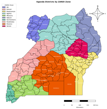
Figure 1. Map of the study area illustrating the spatial distribution of ZARDI regions across Uganda.

Uganda's tropical climate, situated between latitudes 1^°South and 4^° North of the equator, makes it an ideal location for agriculture. The ZARDIs are strategically located in the country's diverse agro-ecological zones, providing tailored agricultural research and support across various regions, as illustrated in the map below

[26]

. Figure 1 presents the geographical distribution of the ZARDI zones across Uganda, showing the country's division into regions with unique environmental conditions. This visual representation underscores significant gradients in climate and landscape traits, highlighting the diverse geography that influences agricultural settings across Uganda

[26]

3.3. Climatic Context of the ZARDI Zones

Uganda's climate is tropical, with two main rainy seasons (March–May and September–December) in most regions. However, northern Uganda experiences a single, longer rainy season (March–October) due to its higher latitude

[34]

. Across the country, mean annual precipitation is ≈1,197 mm (varying 39.6–152.7 mm per month) and mean temperature ≈22.8°C (range ≈21.7°C in July to 23.9°C in February). Maize typically achieves optimal growth with ideal temperatures of 20-22°C during the day and moderate to heavy rainfall of 500-800 mm per month throughout the entire cropping season

[35]

. The yield decreases substantially under stress; for example, both field observations and model output indicate that maize yield drops as temperatures approach approximately 27^°C or as rainfall becomes erratic

[36]

. These physiological sensitivities manifest spatially: the southern and highland zones consistently outperform the north. For instance,

[37]

mapped Uganda’s maize productivity and found two distinct yield zones: a high-yield band (~3.5 t/ha) across central, western, and eastern highlands with moderate temperatures ranging from 20 to 27°C, and lower-yield areas (~1.5 t/ha) in the north (18°C to 35°C), except in some parts of West Nile

[38]

. The local context of Uganda's ZARDI zones demonstrates the balance of these climatic factors

[26]

3.4. Dataset Description

The maize yield datasets used as the dependent variable in this study (measured in tons per hectare) were sourced from the Uganda Bureau of Statistics (UBOS). These data were collected as part of the 50 x 2030 Initiative, an international effort led by the FAO and the World Bank to address agricultural data gaps in 50 countries by 2030. While the Annual Agricultural Survey (AAS) provided standardized, nationally representative data, financial and logistical constraints prevented further follow-up localized surveys within the ZARDI zones after 2020

[26]

. The data span all ZARDI zones for the years 2018 to 2020, aligning with the predictor data timeline. The dataset is geographically stratified by ZARDI, reflecting Uganda’s agro-ecological research zones, which ensures that our model training accounts for spatial and temporal heterogeneity. The use of UBOS, the national custodian of agricultural data, adds credibility, precision, and reliability to the empirically tested maize yield data used herein. Specifically, UBOS employed standardized, validated procedures to conduct AAS, thereby ensuring that the dataset is nationally representative, methodologically consistent, and quality-assured across all ZARDI locations.

We acquired climatic data from the NASA POWER and GPM/IMERG portals at a daily resolution. To correlate this data with maize yield statistics, which are reported biannually (two seasons: Season 1 from February to April and Season 2 from September to December) for each ZARDI zone, we aggregated the daily climatic records into seasonal summaries. For each ZARDI zone and season, we calculated cumulative rainfall, average temperature, average solar radiation, and average soil moisture estimates. Consequently, the final dataset includes 60 observations from 3 years × 2 seasons × 10 ZARDI zones, with each representing a season-level summary. There are no daily yield data for Uganda; therefore, the climatic variables were seasonally aggregated to align with the temporal resolution of UBOS maize yield records (measured in tonnes per hectare). Rainfall and soil moisture serve as primary indicators of water availability, regulating germination and nutrient uptake and alleviating drought stress in plants. Solar radiation supplies the energy required for photosynthesis and biomass production, directly linking climatic energy input to yield potential

[39]

. While Minimum and maximum temperatures regulate enzymatic activity, phenological development, and grain filling, extreme thermal stress often limits yield potential. Collectively, these variables capture the dominant climatic conditions, including atmospheric conditions, water supply and demand, and biophysical drivers of crop productivity

[40, 41]

. For instance,

[39]

found that individual climate variables, such as rainfall, soil moisture, minimum temperatures, and maximum temperatures, contribute approximately 4.2%, 22.5%, 39.2%, and 23.1%, respectively, to the annual variations in maize yield during the growing season in Ghana. The dataset is geographically diverse, covering all ZARDI, allowing for spatial and temporal analysis of maize yield trends. Table 1 summarizes the sources, variables, and spatial-temporal characteristics of the environmental and yield datasets used in this study, providing a clear overview of the inputs to the modelling framework.

Table 1. Data sources and their spatial-temporal features.

Data Type	Variables	Temporal Resolution	Spatial Resolution	Data Source	Link
Weather data	Temperature, solar irradiance, and humidity	Daily (varies)	~0.5° x 0.5° (~50 km)	NASA POWER	https://power.larc.nasa.gov/
Rainfall	Precipitation (IMERG)	2014–present, daily	0.1° x 0.1° (~10 km)	NASA GPM (IMERG)	https://pmm.nasa.gov/resources/documents/gpm-integrated-multi-satellite-retrievals-gpm-imerg-algorithm-theoretical-basis-
Solar radiation	All-Sky Surface Photosynthetically Active Radiation (PAR)	Daily, near real-time	~1° (CERES SYN1deg/FLASHFlux)	NASA CERES & FLASHFlux via POWER	https://ceres.larc.nasa.gov/data/
Soil moisture	Root zone soil wetness (0–100 cm depth)	2014–present, daily	~0.5° (~50 km)	NASA GMAO, MERRA-2 (GEOS DAS)	https://gmao.gsfc.nasa.gov/reanalysis/MERRA-2/

Oversampling was conducted to create a more synthetic dataset of maize yield records using the SMOGN

[28]

. Table 2 below presents the dataset's descriptive statistics before applying SMOGN. This table provides descriptive statistics for seasonal climatic measurements, showcasing the range, mean, and dispersion of values and illustrating the variability and distribution of the underlying data points. This helps improve understanding of how these factors affect the modeling framework.

Table 2. Descriptive statistics of the dataset before applying SMOGN.

FEATURES	Count	Mean	STDEV	Min	25%	Median 50%	75%	Max
SOIL_MOISTURE	60	0.645653	0.155157	0.4075	0.5025	0.64375	0.762708	0.9475
RAINFALL	60	145.7961	56.51327	23.73	116.0163	136.23	170.0681	305.86
SOLAR_RAD	60	134.1094	2.51645	128.4767	132.1969	134.1125	136.0406	138.66
MAX_TEMP	60	28.94388	2.944299	23.79	26.53333	28.16625	31.45625	35.2725
MIN_TEMP	60	15.64457	2.200786	11.1825	13.80313	16.2475	17.34833	19.4
YIELD	60	1.698333	0.635794	0.6	1.3	1.6	2	4

3.5. Data Pre-processing

Data preprocessing was a crucial step in preparing the dataset for robust, reliable yield prediction in maize. Handling missing values in this dataset involved imputing the median value for numerical features, such as soil moisture, rainfall, solar radiation, maximum temperature, and minimum temperature, to avoid losing valuable records. The categorical ZARDI zones were numerically encoded using label encoding, making them suitable for ML models while preserving each zone's unique identity. This was followed by standardizing the continuous features using StandardScaler

[42]

, which normalizes feature values to have a mean of zero and a standard deviation of one, thereby ensuring uniform scaling across all features. Then, interaction terms were developed using the Polynomial Features transformation to analyze the combined climatic impacts on maize physiology. These terms resulted from multiplying standardized values of the variables, for example, Rainfall_MaxTemp = Rainfall_scaled x MaxTemp_scaled. This approach indicates that maize yield is influenced by the interaction among climatic factors rather than by individual variables. The combination of Rainfall_scaled and Solar radiation addresses the effects of water availability and energy input on crop growth. All interaction features are established during pre-processing and incorporated into the model as fixed predictors, eliminating the need for runtime adjustments. As a result, throughout the ten ZARDI zones, the yield records were temporally and spatially sparse. This is demonstrated in the pseudocode in Table 3, which outlines the key preprocessing steps

[43]

Table 3. Pseudocode for the Data Pre-processing Pipeline.

Step	Description
Input	Maize yield data (2018–2020) and environmental variables (soil moisture, rainfall, solar radiation, maximum and minimum temperature).
Output	Pre-processed training and testing datasets.
1. Data acquisition	Collect maize yield data from UBOS and environmental data from NASA POWER.
2. Data cleaning	Impute missing values (median for continuous, mode for categorical), remove duplicates, and drop implausible records.
3. Categorical encoding	Apply label encoding to ZARDI zones to make them suitable for ML models while preserving zone identity.
4. Outlier handling and scaling	Apply StandardScaler to normalize continuous variables (mean = 0, standard deviation = 1).
5. Feature engineering	Generate higher-order interaction terms using Polynomial Features to capture complex climatic relationships.
6. Partitioning	Split into training (80%) and testing (20%) sets, stratified by ZARDI zone. Validate subsets for completeness and representativeness.

For continuous climatic variables, missing observations were imputed using medians to address skewness and extreme events commonly observed in environmental data across various ZARDI zones. Median imputation is advantageous as it is resistant to extreme values, preserving the characteristics of existing observations. For categorical variables, mode imputation was utilized to accurately assign geographical areas to their respective zones based on ZARDI codes. To maintain data integrity, duplicates across datasets were removed to prevent distortion of seasonal patterns. Furthermore, observations exceeding agronomically feasible thresholds were excluded, ensuring that only realistic environmental data and maize yields were utilized in subsequent analyses and modeling. Furthermore, interpolation was inappropriate in this context because the missing data resulted from spatial rather than temporal inconsistencies. This shows that using interpolation would make unwarranted assumptions not supported by the underlying data-generating process. The final dataset was split into training and test sets at an 80:20 ratio to ensure good generalization and unbiased model performance. This split strategy, widely used in yield prediction studies, strikes a balance between the need for sufficient training data and the requirement for reliable evaluation on the test set. Within the training set, we performed five-fold cross-validation to optimize model parameters and assess variability. This approach maximizes the use of the limited data while guarding against overfitting. The resulting pre-processed dataset, enriched with synthesized data and feature engineering, captured environmental variability. This robust foundation supports the development of cutting-edge ML models with high predictive accuracy for maize yields across diverse agro-ecological regions in Uganda. The following section describes SMOGN oversampling as a crucial preprocessing step to improve the model's performance.

3.6. Smogn Oversampling for Imbalanced Yield Regression Data

The lack of observations at the extremes of the target variable's distribution, such as very low or very high yields, hampers the model's ability to learn those conditions

[28]

. SMOGN was applied as a pre-processing step to balance the yield distribution. It generates new samples in under-represented regions by interpolating between minority examples and their nearest neighbours, then adding Gaussian noise to increase variability. SMOGN also performs a mild under-sampling of the class to avoid biasing the model towards the middle of the distribution. We preferred SMOGN over simpler oversampling methods, such as SMOTER alone, because it better preserves continuous target relationships and has demonstrated superior performance on small, imbalanced regression datasets

[44]

. The process involves importing the original dataset, applying SMOGN to create a balanced dataset, and then training the model on the resulting balanced data

[28]

. The pseudocode for the SMOGN technique is shown in Algorithm 1

[45]

Algorithm 1. Pseudocode for SMOGN

1) Initialize SMOGN parameters (oversampling ratio, Gaussian noise parameters, k for k-nearest neighbours)

2) For iteration = 1 to the number of iterations, do

3) Identify the minority samples in the training data based on the target variable

4) For each minority sample, do

5) Use k-nearest neighbors to find the closest sample to the minority sample

6) Randomly select one of the k-nearest neighbours

7) Generate a synthetic sample by interpolating between the minority sample and the selected neighbour

8) Add Gaussian noise to the synthetic sample to make it more realistic

9) End For

10) Combine the original training data with the synthetic samples to create a balanced training dataset

11) End For

12) Return the balanced training dataset

After implementing SMOGN, the training dataset expanded from 60 to 295 samples, effectively representing both extremely high and extremely low maize yields. The oversampling concentrated on enhancing the representation of sparse yield ranges, particularly for yields below 1.0 t/ha and above 2.5 t/ha. The descriptive statistics in Table 4 reveal that the augmented dataset achieves a more balanced yield distribution than the original dataset (Table 2), with a slight increase in the standard deviation of the target variable, indicating improved coverage of both low- and high-yield conditions. Crucially, the mean values and quartiles of the climatic predictors and yield variables remain nearly consistent with their original values, demonstrating that SMOGN successfully balanced the previously underrepresented yield ranges while preserving their marginal distributions.

Table 4. Presents descriptive statistics of the dataset after applying SMOGN.

FEATURES	Count	Mean	Std	Min	25%	50%	75%	Max
SOIL_MOISTURE	295	0.644403	0.151008	0.4075	0.507375	0.63975	0.75725	0.9475
RAINFALL	295	143.3887	56.64988	23.73	112.8571	136.23	165.2947	305.86
SOLAR_RAD	295	134.0808	2.539926	128.4767	132.1322	134.1272	136.0005	138.66
MAX_TEMP	295	28.93428	2.889725	23.79	26.53	28.2	31.1	35.2725
MIN_TEMP	295	15.64743	2.140631	11.1825	13.8	16.23	17.2	19.4
YIELD	295	1.730725	0.686363	0.6	1.289	1.611	2.018	4

The goal was to achieve a more uniform distribution by generating synthetic data, employing precise parameter tuning with k=5 neighbors and a Gaussian noise level of 0.01. This involved 100% oversampling of minority instances, as outlined by Branco et al

[28]

. Stringent constraints were imposed on synthetic yields to prevent unrealistic values, thereby avoiding negative yields and limiting them to levels near established agronomic maxima, thereby ensuring data realism throughout the augmentation process. For instance, the synthetic yields were constrained to a biologically plausible range of 0.5 to 4.5 t/ha, aligning with agronomic conditions observed in Uganda. The subsequent dataset was split into training and test sets at an 80/20 ratio, yielding 236 training and 59 test samples. Among these, 187 training and 47 test instances were synthetic, ensuring balanced representation of rare yield cases.

To validate the realism of the SMOGN-augmented yield data, various visual and statistical diagnostics were employed, including an examination of marginal distributions of real and synthetic yields. This validation utilized yield distribution plots, quantile–quantile plots, and two-sample tests like Kolmogorov-Smirnov, confirming that the shape, spread, and central tendencies of the synthetic data were closely aligned with those of the original data

[46, 47]

. Notably, there were no significant distortions in basic summary statistics such as means, variances, and percentiles. However, the distribution following SMOGN implementation was more uniform, consistent with the natural trends of the original dataset. This further reinforced the integrity of the augmented data, validating the absence of extreme outliers and demonstrating a more controlled representation of minority regions in the feature space

[48]

. As a result of this pre-processing step, the dataset’s imbalance was significantly reduced while maintaining a realistic feature-target relationships approach validated in recent studies

[27, 45]

3.7. Proposed Ensemble Model

The maize yield prediction framework integrates Decision Tree (DT), Random Forest (RF), and LightGBM to balance interpretability, robustness, and predictive performance within a nonlinear agricultural modeling context. A Decision Tree partitions the feature space into homogeneous regions by minimizing prediction error, making it well suited to capturing complex interactions among climatic variables and soil properties

[49]

. However, single trees are prone to high variance and overfitting. Random Forest (RF) addresses this limitation by using bootstrap aggregation and random feature selection, constructing multiple uncorrelated trees and averaging their predictions to reduce variance and improve generalization. This ensemble mechanism enhances model stability, particularly when dealing with noisy and heterogeneous agricultural datasets

[50]

LightGBM further enhances predictive performance by employing a gradient-boosting framework that sequentially builds trees to minimize residual errors. Its histogram-based feature binning reduces memory consumption and accelerates training, while its leaf-wise tree growth strategy improves accuracy by focusing on splits that yield the highest information gain. Additionally, built-in regularization mechanisms help control model complexity and mitigate overfitting

[51]

. These properties make LightGBM particularly suitable for large-scale agricultural datasets derived from weather records and satellite imagery. The final weighted ensemble combines the complementary strengths of DT (interpretability), RF (variance reduction and robustness), and LightGBM (high predictive accuracy and scalability), resulting in improved stability, reduced overfitting risk, and enhanced generalization performance in maize yield forecasting

[52]

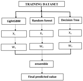
Figure 2 shows the architecture of the weighted ensemble method, in which climatic and categorical variables are simultaneously fed into three base learners: LightGBM, RF, and DT. Each learner produces yield predictions xj (j=1, 2, 3), which are then aggregated using a layer that applies fixed weights. These weights wj (j=1, 2, 3) are derived from the inverse-RMSE normalization method applied to the validation set

[49]

. These weighted outputs are then aggregated in the ensemble layer to generate the final prediction, as shown below.

Download: Download full-size image

Figure 2. Structure of the weighted average ensemble

[53]

The final model weights are determined by initializing three base models, each with equal weights of

w_{j}

\frac{1}{3}

. These preliminary weights were refined using an inverse-RMSE normalization procedure during five-fold cross-validation rather than assigned heuristically. For each model j, the weight was computed as in equation (1)

[49, 54]

w_{j} = \frac{{RMSE}_{j}^{- 1}}{\sum_{k = 1}^{m} {RMSE}_{k}^{- 1}}

(1)

Where m is the number of models and k is the index representing each model in the ensemble. The RMSEj is the Root Mean Squared Error of the j-th model computed on the validated datasets. This formulation ensures proper weight normalization and allocates greater influence to models exhibiting lower predictive error. Using this procedure, the resulting weights include: LightGBM = 0.3333, RF = 0.3345, and Decision Tree = 0.3322, which were then fixed for inference. The average is obtained by multiplying each base learner's prediction (x_j) by its corresponding weight (w_j)

[55]

. The final ensemble model was computed in equation (2)

[49, 56]

final predicted value = \frac{\sum_{j = 1}^{m} w_{j} x_{j}}{\sum_{j = 1}^{m} w_{j}}

(2)

Where m denotes the number of models to be averaged, w_j stands for assigned weights, and

x_{j}

is the prediction from the j^th model.

The weighted average approach balances low-prediction-error models in the ensemble while preserving the benefits of model diversity, allowing the strengths of different components to complement one another within the assembled ML model and thereby ensuring overall model performance. In addition to improving its predictive accuracy, the technique made the model more stable by mitigating weaknesses associated with using individual models

[56, 57]

. This explains why it performed exceptionally well among standalone models, achieving excellent metrics and generalization across all ZARDI zones in Uganda.

3.8. Performance Metrics

The performance of the proposed ensemble model was evaluated using four key metrics: Mean Absolute Error (MAE), Mean Squared Error (MSE), RMSE, and R² score. These metrics can be used comprehensively to assess the model's predictive accuracy. The MAE was chosen for its intuitive interpretation as the average magnitude of prediction errors, providing a simple measure of prediction accuracy without overweighting larger errors

[58, 59]

. MSE was included because it squares the prediction errors, thereby emphasizing larger prediction errors and being especially useful for identifying models that minimize significant deviations

[29, 60]

. The MSE is converted to RMSE, which presents error values in the same units as the target variable, maize yield, making them easier to interpret and more practical

[61]

. Lastly, the R² score was selected to examine the proportion of variance in maize yield explained by the model

[62]

. It indeed provided a normalized measure of predictive power that accounted for dataset variability

[13]

. It follows that these metrics provide a balanced assessment of the model's accuracy and reliability, thereby enhancing the robustness of the ensemble performance validation over Uganda's ZARDI zones. The MAE, MSE, RMSE, and R² Score are shown in Equations (3)-(6), respectively.

MAE = \frac{1}{n} \sum_{i = 1}^{n} | y_{i} - ŷ_{i} |

(3)

MSE = \frac{1}{n} \sum_{i = 1}^{n} {(y_{i} - ŷ_{i})}^{2}

(4)

RMSE = \sqrt{\frac{1}{n} \sum_{i = 1}^{n} {(y_{i} - ŷ_{i})}^{2}}

(5)

R^{2} = 1 - \frac{\sum_{i = 1}^{n} {(y_{i} - ŷ_{i})}^{2}}{\sum_{i = 1}^{n} {(y_{i} - {\overset{̅}{y}}_{i})}^{2}}

(6)

Where:

yᵢ: Actual value for the i-th observation

ŷᵢ: Predicted value for the i-th observation

ȳ: Mean of the actual values

n: Total number of observations

3.9. Model Implementation

The proposed ensemble model for predicting maize yield was implemented in Google Colab, a cloud-based platform that enables easy collaborative coding and powerful computing. This model was implemented in Python 3.10, utilizing Pandas and NumPy for data manipulation and preprocessing, Scikit-learn for model training and evaluation, and Matplotlib for visualization. Pre-processing steps included scaling continuous features using StandardScaler to ensure consistent scaling across variables. The dataset was split 80-20 into training and test sets to ensure unbiased evaluation. LightGBM, Random Forest, and Decision Tree were then trained using their respective regressor classes, with hyperparameter tuning to ensure optimal performance. The metrics used to evaluate model performance are MAE, MSE, RMSE, and R². Each model has been combined into an ensemble using a weighted average of its predictions, with weights determined by its performance metrics. Predictions and visualizations of maize yield trends have been generated, providing actionable insights into climatic impacts across ZARDI zones. The interactive environment and pre-installed libraries in Google Colab made the implementation efficient and reproducible.

3.10. Model Hyperparameters and Implementation Details

This study employed ML and DL models to predict maize yield across Uganda's agroecological zones. We provide detailed descriptions of dataset size, model architectures, hyperparameter tuning processes, and optimization techniques to support replicability and model reliability. For ML models, including LightGBM, RF, and Decision Tree, we used 295 records obtained after applying the SMOGN technique to balance the original yield data. We implemented hyperparameter tuning using a grid search with five-fold cross-validation. This process enabled us to systematically explore parameter combinations and select the best-performing configurations based on validation performance. For RF, the best results were achieved with 200 trees, a maximum depth of 20, and a minimum sample split of 2. The Decision Tree model performed best at depth 15 with 2 samples per leaf, while the LightGBM model was optimized with 200 estimators, a learning rate of 0.05, and a depth of 10. All ML models were implemented using the scikit-learn library in Python, and model performance was evaluated using R² and RMSE metrics. These metrics were calculated using the held-out test set to ensure an objective evaluation.

The DL model was implemented by organizing the dataset into a time-series of seasonal climatic profiles, which is suitable for analysis using CNN and LSTM architectures. The CNN model's architecture was designed to recognize spatiotemporal patterns in climate time-series data. Two 1D convolutional layers with 32 and 64 filters and a kernel size of 2, each followed by a ReLU activation, were succeeded by a max-pooling layer and a dense output layer. In contrast, the LSTM model focuses on the temporal dependencies within the sequence data. Its architecture comprised two stacked LSTM layers, with sizes of 64 and 32, respectively, and a final dense layer for regression output. The LSTM model employed the tanh activation function for the internal cell state, while the gate activation function was sigmoid.

LSTM and CNN were trained with a batch size of 8, the Adam optimizer with a learning rate of 0.001, and mean squared error (MSE) loss, which is appropriate for regression tasks. The training was conducted in batches of 8 samples, in line with the established batch size. A dropout layer with a rate of 0.3 was used during training to prevent the model from relying too heavily on specific neurons.

Additionally, early stopping was applied during training, with the process halted when the validation loss failed to improve for 10 consecutive epochs. To optimize model performance, hyperparameter tuning was performed via grid search, enabling identification of the best configuration for each model. An upper limit of 100 epochs was set in the early-stopping protocol, although convergence typically occurred between 70 and 85 epochs. Subsequent testing at epochs 50, 150, and 200 did not yield any performance improvements, thereby validating the chosen configuration. These strategies were effective in reducing the risks of model overfitting. The data was transformed into the three-dimensional format required by CNN and LSTM models, with the form (samples, time steps, features). This was done to maintain the temporal and spatial relationships in the climatic data, enabling effective learning by the DL models. A consistent test data split was used across all models to ensure a fair and accurate comparison of their predictive performance. A 20% validation split was used during training to monitor generalization performance. All DL experiments were conducted using TensorFlow, and the Keras API ensured transparency and reproducibility. This detailed modeling setup enabled us to fine-tune model parameters and extract meaningful patterns from complex climate and yield data, resulting in robust maize-yield predictions. The model's hyperparameters and implementation details are provided in Table 5 below.

Table 5. The model's hyperparameters and implementation details.

Component	Model Implementation Specification
Dataset	295 records (SMOGN balanced), time-series format with seasonal climatic profiles
Models Used	ML: LightGBM, Random Forest (RF), Decision Tree (DT) DL: CNN, LSTM
Implementation	ML: scikit-learn DL: TensorFlow with Keras API
Hyperparameter Tuning	Grid search (with 5-fold cross-validation for ML)
ML Model Details	RF: 200 trees, depth = 20, min split = 2 DT: depth = 15, min samples/leaf = 2 LightGBM: 200 estimators, LR = 0.05, depth = 10
DL Architecture	CNN: 2 × 1D Conv layers (32, 64 filters, kernel = 2), ReLU, max-pooling, dense output LSTM: 2 layers (64, 32 units), tanh/sigmoid, dense regression output
DL Training Settings	Batch size = 8, learning rate = 0.001, optimizer = Adam, loss = MSE, 20% validation split
Regularization	Dropout = 0.3, early stopping (patience = 10, max epochs = 100)
Input Format	3D tensor: (samples, time steps, features)
Evaluation Metrics	R², RMSE (for both ML and DL models)
Comparison Strategy	Consistent test data split used across all models for fair evaluation.

4. Experimental Results

4.1. Comparative Performance of Machine Learning Models

The performance metrics in Table 6 reveal a significant difference in the predictive capability of the models tested for maize yield (tons per hectare). Random Forest and LightGBM outperformed all the other models. Random Forest had the smallest MAE (0.04 tonnes), MSE (0.00 tonnes²), and RMSE (0.07 tonnes), while achieving an R² of 0.99, which explains almost all of the variance in the yield data. LightGBM performed very well, too: 0.05 tonnes for MAE, 0.01 tonnes² for MSE, 0.08 tonnes for RMSE, and 0.99 for the R² score. It is worth noting that the Decision Tree performed exceptionally well, too: the MAE is 0.03 tonnes, the MSE is 0.01 tonnes², the RMSE is 0.09 tonnes, and the R² score is 0.98 - although a bit less potent in comparison with RF and LightGBM in terms of minimizing the error of a single prediction. A comprehensive comparative analysis on tabular data was conducted using two deep learning (DL) algorithms: a 1D Convolutional Neural Network (CNN) and a Long Short-Term Memory (LSTM) network. Recent experiments have shown that DL techniques, including CNNs and LSTMs, are effective in capturing crop characteristics throughout the growing season. 1D-CNNs can extract nonlinear spatial features from structured climate inputs, such as spatially correlated rainfall or temperature grids. Conversely, LSTMs focus on capturing phenological and temporal dependencies, which allows them to model sequential crop responses to changing climatic conditions

[32, 60]

. Support vector regression (SVR) and linear models such as Ridge and Lasso were excluded from the analysis because of the strong nonlinearity in the ZARDI-scale maize-yield series, which linear models cannot adequately address. Specifically, an SVR using radial basis function (RBF) kernels exhibited significant instability and high parameter sensitivity when applied to the SMOGN-enhanced dataset. As a result, decision tree models were preferred for their superior robustness, stability, and interpretability, making them particularly suitable for use with smaller agricultural datasets. Although the dataset's sample size was limited, it enhanced the analysis. Deep learning models performed moderately: the CNN achieved an R² of 0.83, whereas the LSTM achieved 0.79, indicating lower efficacy in capturing complex relationships than tree-based models. Both also had higher error metrics: the CNN's RMSE was 0.27 tonnes, while the LSTM's was 0.30 tonnes. Given the strong performance of Decision Tree, Random Forest, and LightGBM, an ensemble model was constructed using these three models to leverage their complementary strengths.

Table 6. Performance Summary of ML Models.

Model	MAE (tonnes)	MSE (tonnes²)	RMSE (tonnes)	R² Score
CNN	0.18	0.07	0.27	0.83
LSTM	0.19	0.09	0.30	0.79
Decision Tree	0.03	0.01	0.09	0.98
Random Forest	0.04	0.00	0.07	0.99
LightGBM	0.05	0.01	0.08	0.99

4.2. Performance of the Proposed Ensemble with Base Models

The performance results in Table 7 reveal that the base models LightGBM, Random Forest, and Decision Tree (DT), as well as the ensemble model, demonstrated strong predictive performance for maize yield. The DT provides transparent rules and ensemble methods, such as RF and LightGBM, that capture nonlinearities and interactions and provide explicit feature importance. Of all the base models, the Random Forest had the lowest error metrics: a MAE of 0.04 tonnes, a MSE of 0.00 tonnes², and an RMSE of 0.07 tonnes, while achieving an R² score of 0.99. LightGBM also did very well with a MAE of 0.05 tons and an R² score of 0.99, while the Decision Tree model developed the lowest MAE, at 0.03 tons, but a little higher in RMSE (0.09 tons), with a slightly lower R² score of 0.98. The ensemble model outperformed the individual models, achieving the lowest RMSE of 0.06 tonnes and an R² of 0.99. This indeed provides evidence that the ensemble effectively leverages the complementary strengths of the base models, thereby improving prediction accuracy and stability. The near-equal weights of the models in the ensemble further reflect their balanced contributions, making the ensemble the most reliable approach to predicting maize yield across Uganda's ZARDI zones.

Table 7. Performance of Base Models and Ensemble.

Model	MAE (tonnes)	MSE (tonnes²)	RMSE (tonnes)	R² Score
LightGBM	0.05	0.01	0.08	0.99
Random Forest	0.04	0.00	0.07	0.99
Decision Tree	0.03	0.01	0.09	0.98
Proposed Ensemble	0.03	0.00	0.06	0.99

These three models were selected as the baseline for predicting maize yield in Uganda. The chosen models are applicable and relevant to the available data. Given the dataset's limited size (≈60 samples, augmented to ~295) and its structured format, we restricted our model selection to ensure interpretability and accuracy. We excluded algorithms such as linear regression because they tend to overfit or cannot capture complex nonlinear climate–yield interactions. Models such as CNNs and LSTMs were used as base models because they have been extensively used for spatial-temporal yield prediction. However, they underperformed (R²≈0.79–0.83) compared to tree ensembles (R²≈0.99), due to the limited number of structured datasets, making traditional ensemble learners more suitable for the study’s context. XGBoost was not used because it has equal strengths to LightGBM. This model selection strikes a balance between high accuracy, efficiency, and interpretability for our data-confined maize yield prediction task.

4.3. Maize Yield Predictions

Table 8 presents maize yield predictions for 2018-2020, comparing forecasts from individual models and a proposed ensemble method with observed yields. Each row distinguishes among unique ZARDI combinations and seasonal contexts, underscoring the importance of the temporal dimension. The ensemble method, which integrates LightGBM, RF, and DT models, achieves higher accuracy in predicting moderate-to-high yields than standalone models. These findings align with the error analyses presented in Tables 6 and 7 and explain the benefits of model integration. For example, the ensemble predicts an actual yield of 1.309 tonnes, which is 1.306 tonnes, thereby minimizing inter-zone deviation. Similarly, for an actual yield of 1.701 tonnes, the ensemble predicted 1.698 tonnes, indicating strong regional adaptability. The baseline models, such as Random Forest and LightGBM, while exhibiting minor variations in some cases, underpredict yields in specific zones; for instance, Random Forest predicted an actual yield of 2.306 tonnes as 2.082 tonnes. However, this ensemble avoids such biases by leveraging the strengths of each model to provide more accurate and stable predictions, even when the dataset spans multiple agricultural zones with potentially different climatic and environmental factors. The ensemble's performance across mixed zones speaks volumes to its versatility, especially in applications within regionally diverse agricultural settings. This ability to generalize across zones while maintaining high predictive accuracy underlines its utility for yield forecasting and decision-making in multi-regional agricultural planning.

Table 8 presents a representative subset of in-season maize yield estimates from 2018 to 2020, comparing individual forecasting models, an ensemble approach, and the actual yields recorded during those seasons. Notably, the ensemble method yielded predictions that closely aligned with the actual yields, surpassing other individual models. In the performance analysis, CNN and LSTM models were excluded due to their significantly lower accuracy, with R² values around 0.79 to 0.83. In contrast, tree-based models demonstrated much higher accuracy, with R² values of approximately 0.99, making them more suitable for this ablation-style analysis given the limitations of the dataset's size and structure.

Table 8. Shows some of the Maize Yield Predictions: Actual vs. Model Outputs.

Actual Yield (tonnes)	LightGBM (tonnes)	Random Forest (tonnes)	Decision Tree (tonnes)	Ensemble (tonnes)
1.309242	1.295747	1.313376	1.308188	1.305777
2.306264	2.234435	2.082308	2.308199	2.208053
1.897813	1.894917	1.900684	1.89184	1.895824
1.903575	1.918706	1.895232	1.9	1.90464
1.995159	2.004441	1.997771	2.00408	2.00209
0.898441	0.950394	0.963395	0.89226	0.935431
1.988837	2.053294	2.003895	1.996994	2.018067
1.892176	1.868493	1.902487	1.917591	1.896175
1.001636	1.004797	0.997463	0.991298	0.997859
2.403842	2.389707	2.401232	2.410852	2.400586
1.894133	1.878223	1.837471	1.905315	1.873591
1.798547	1.792779	1.797281	1.80665	1.798893
1.701368	1.700425	1.697947	1.694446	1.69761

4.4. Feature Importance in the Prediction of Maize Yields

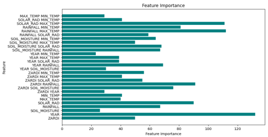
Figure 3 ranks the predictors based on their contributions to the ensemble model. Seasonal soil moisture, rainfall, and solar radiation are the most critical climatic drivers, while the “Year” and “ZARDI” variables reflect greater temporal and spatial variability in agronomic conditions. Interaction features contribute moderately, indicating that combined climate effects are significant but secondary to the primary climatic variables. The feature importance analysis demonstrates that ‘Year’ is the most influential predictor of maize yield variability in Uganda, reflecting substantial interannual fluctuations that are not fully captured by the individual climatic variables. As an integrative temporal variable, ‘Year’ embodies shifts in rainfall patterns, temperature regimes, agronomic practices, and broader socio-economic conditions that change from one season to the next. Changes in the environment and management from season to season collectively have a significant impact, though this effect is not directly reflected in the dataset. Its prominence, therefore, reflects genuine temporal variability in maize yields rather than model bias, consistent with findings from related crop-yield modelling studies. This indicates that "Year" serves as a proxy for various factors that significantly influence maize productivity over time. Similarly, the ZARDI zones in Uganda exhibit significant predictive capacity for estimating maize yields, as they accurately reflect variations in geographic and climatic factors. Each zone corresponds to unique differences in rainfall, temperature, and agricultural management practices that influence land suitability for maize production. Consequently, the ZARDI variable serves as a reliable spatial indicator of these environmental factors that shape maize productivity.

Download: Download full-size image

Figure 3. Feature Importance in the Prediction of Maize Yields.

Among all the climatic variables, soil moisture, rainfall, and solar radiation are the most impactful, reflecting their critical role in crop growth and development. Furthermore, the temperature variables, particularly MAX_TEMP and MIN_TEMP, are crucial because they influence plant stress and growth conditions. Some interaction terms, such as Rainfall × Solar radiation and Soil moisture × Solar radiation, indicated that it is not just one climatic factor but several combined factors that ultimately affect maize yield. However, these are not as influential as individual ones. Overall, the results emphasized the need to consider spatial, ZARDI, and temporal-year variability, along with key climatic factors, when developing robust models to predict maize yield. These findings confirm that comprehensive datasets reflecting regional and temporal differences are essential for agricultural forecasting.

4.5. The Distribution of Residuals in the Detection of Bias of Our Proposed Ensemble

Download: Download full-size image

Figure 4. The Distribution of Residuals with our Proposed Model.

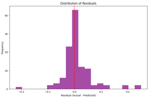
Figure 4 presents a histogram of the residuals (Actual - Predicted). This histogram will provide a sense of the predictive model's accuracy. Residuals centre around zero, as indicated by the red dashed line at 0, suggesting that this model is not significantly biased in making its predictions. The symmetrical, bell-shaped distribution suggests that the bulk of the residuals are close to zero; hence, the predicted values are generally accurate and agree well with the actual maize yields. The general spread of residuals is narrow, with only a few exceeding ±0.1, reflecting the model's consistency and reliability in minimizing significant prediction errors. There are no extreme outliers, further supporting the model's strength. This overall residual analysis therefore confirms that the model has captured the data's underlying patterns and thus minimizes systematic error, making it suitable for accurate maize yield prediction across different ZARDI zones.

4.6. Effect of SMOGN Augmentation on Model Performance

This subsection analyzes the influence of SMOGN-based augmentation on model accuracy. Although SMOGN increases the representation of rare yield values, it does not introduce new agronomic relationships between climatic variables and yield outcomes; therefore, its value must be demonstrated empirically. To this end, the performance of the three principal base learners, LightGBM, Random Forest, and Decision Tree, was evaluated both before augmentation using the original 60 observations and after augmentation using the expanded set of 295 samples. Table 9 presents the results and shows that all three models exhibit notable improvements in predictive accuracy following augmentation. Random Forest improves from an R² of 0.85 before augmentation to 0.99 afterwards, accompanied by a reduction in RMSE from 0.18 t/ha to 0.07 t/ha. LightGBM demonstrates a similar pattern, with R² increasing from 0.82 to 0.99 and RMSE decreasing from 0.20 t/ha to 0.08 t/ha. Decision Tree performance also strengthens markedly, improving from an R² of 0.74 to 0.98 while RMSE drops from 0.25 t/ha to 0.09 t/ha. These gains confirm that SMOGN enhances the model’s ability to learn patterns across the full spectrum of yield variability, particularly in previously underrepresented low- and high-yield regions.

The results further reveal that augmentation primarily enhances internal consistency rather than generalizable real-world performance. Because approximately 80% of the dataset becomes synthetic after augmentation, model performance reflects improved distributional balance rather than verified predictive skill on independent yield records. This limitation has been explicitly acknowledged, and the study recommends that future work incorporate temporal or spatial hold-out validation using real field-collected yield data. Such validation will be essential for assessing whether the improvements observed after SMOGN augmentation extend beyond the controlled experimental environment.

Table 9. Performance of Base Models Before and After SMOGN Augmentation.

Model	R² (Before)	R² (After)	RMSE Before (t/ha)	RMSE After (t/ha)
LightGBM	0.82	0.99	0.20	0.08
Random Forest	0.85	0.99	0.18	0.07
Decision Tree	0.74	0.98	0.25	0.09

4.7. Uncertainty Estimation and Predictive Confidence Intervals

Although the proposed ensemble model demonstrates high predictive accuracy, the current study did not compute uncertainty estimates or confidence intervals around the predictions. This omission is significant because ensemble-based yield forecasts derived from small, synthetically augmented datasets may be more sensitive to sampling variability. Confidence intervals, such as those derived from nonparametric bootstrapping or Monte Carlo simulations of ensemble members, are essential for quantifying the reliability and stability of predicted yields, particularly in regions with sparse observations. Given the limited temporal span (2018–2020) and the heavy reliance on SMOGN-generated yield values, applying rigorous uncertainty quantification within the present analysis would risk producing misleading or artificially narrow intervals. We therefore acknowledge that the absence of predictive intervals represents a methodological limitation of this study. Future work should incorporate formal uncertainty estimation methods, such as residual bootstrapping, ensemble resampling, quantile regression forests, conformal prediction, or Bayesian ensemble modeling, to provide probabilistic yield forecasts and more robust decision-support for agricultural stakeholders.

5. Discussion of Results

The experimental results indicate that the ensemble model combining LightGBM, Random Forest, and Decision Tree achieved the most consistent predictive performance among the evaluated approaches. The ensemble attained an R² of approximately 0.99 with a root mean squared error (RMSE) of about 0.06 t/ha, outperforming the individual tree-based models whose RMSE ranged from about 0.07 to 0.09 t/ha. In contrast, the deep learning models produced substantially lower explanatory performance (R² ≈ 0.79–0.83) and higher prediction errors (RMSE ≈ 0.27–0.30 t/ha). These results demonstrate that aggregating complementary tree-based learners improves predictive stability in structured agricultural datasets. Similar improvements from ensemble approaches have been reported in crop-yield modelling studies, where multiple learners reduce variance and improve generalization

[30, 33]

Despite the strong numerical performance, the results must be interpreted carefully. The original dataset consisted of only 60 real seasonal observations collected between 2018 and 2020, and the training data were expanded to 295 samples using SMOGN-based synthetic oversampling. Under such conditions, very high goodness-of-fit values may reflect improved internal consistency rather than confirmed real-world predictive accuracy. Previous studies have noted that augmentation techniques can substantially improve learning behaviour in small regression datasets, but do not necessarily guarantee external generalization

[27, 63]

. Therefore, the reported R² should be interpreted as demonstrating modelling feasibility under limited data rather than as evidence of operational yield-prediction capability.

The improvement observed after SMOGN augmentation further supports this interpretation. Before augmentation, the models exhibited lower explanatory power, whereas after balancing rare yield values, the performance increased markedly. This suggests that the primary limitation to learning was the sparsity of data on extreme yield conditions. Nevertheless, synthetic observations cannot substitute independent field measurements, and the model requires validation using additional years of data before deployment in decision-support settings.

Feature-importance analysis indicated that soil moisture, rainfall, and solar radiation were the most influential predictors of yield variability. These variables directly relate to crop water availability and photosynthetic energy supply, which are well-established determinants of maize growth

[39-41]

. The strong influence of the temporal variable (“Year”) likely reflects seasonal variability and unobserved agronomic factors, including management practices and localized climatic variability, that the available predictors did not capture.

The lower performance of deep learning models compared to tree-based ensembles is also consistent with previous research. Deep neural networks typically require large training datasets, whereas decision-tree ensembles are better suited to structured tabular datasets with limited observations

[32, 60]

. In agricultural studies characterized by small and heterogeneous datasets, ensemble learners therefore remain more appropriate modelling tools.

Therefore, the findings indicate that ensemble learning, combined with controlled synthetic augmentation, can extract meaningful patterns from limited agricultural records. However, independent temporal or spatial validation is necessary before the approach can be considered reliable for real-world agricultural decision-support applications.

5.1. Practical Implications of the Study

The study shows that a weighted ensemble model combined with SMOGN oversampling can predict maize yields even with very limited data. In Uganda’s diverse agro-ecological zones (and similar regions), this approach achieved high accuracy, proving that yield prediction is feasible under data scarcity. While still a proof-of-concept rather than an operational tool, the method offers several actionable insights for agricultural policy, farm management, and early warning systems:

1) Yield Forecasting with Minimal Data: The successful use of SMOGN (synthetic oversampling) to expand a tiny dataset (from 60 to 295 samples) illustrates how other data-scarce countries can build yield models. By generating synthetic data points for underrepresented scenarios, early-warning agencies can train machine-learning models to forecast harvests even when historical records are sparse. This methodology enables more quantitative crop outlooks in regions that currently rely on limited surveys or expert judgment.

2) Focus on key yield drivers: The model confirms that water and temperature are the primary determinants of maize yields. Extension programs can emphasize practical techniques for farmers to optimize these factors, such as soil moisture conservation (e.g., mulching, rainwater harvesting) and timely planting to synchronize crop growth with peak periods of rainfall and sunlight. By acting on these data-driven insights, farmers can enhance yield potential even in challenging seasons.

3) Improved national yield forecasts: Governments can integrate an ensemble-based yield model into crop-monitoring systems to generate early-season yield forecasts. Even a rough pre-harvest estimate allows policymakers to plan grain storage, imports, or relief distribution in advance, strengthening food security planning.

4) Decision support for farmers: Once validated, the ensemble model could be used in farmer advisory apps or extension services to provide localized yield forecasts. Mid-season predictions (based on rainfall, soil moisture, and related variables) would help farmers make critical decisions, such as adjusting fertilizer use, planning irrigation during dry spells, or timing the harvest, to improve outcomes and reduce potential losses.

5.2. Limitations and Future Work

Although the proposed ensemble modelling approach demonstrated strong performance within the experimental dataset, several limitations must be acknowledged.

First, the study relied on a very limited number of real observations. The maize yield dataset contained only 60 seasonal records spanning the period 2018–2020. To address severe imbalance and data sparsity, SMOGN-based synthetic oversampling expanded the dataset to 295 samples. While this improved model learning behaviour and internal predictive consistency, synthetic observations cannot replace independent field measurements. Consequently, the reported predictive performance reflects model behaviour within an augmented distribution and should not be interpreted as validated real-world forecasting accuracy.

Second, the dataset's temporal coverage was limited. Agricultural productivity is influenced by interannual climate variability, agronomic practices, pest pressure, and localized management conditions. Because the available data covered only three years, the model may not capture long-term climatic variability. External validation using additional years of data (e.g., 2021 onward) or independent field observations is therefore necessary before practical deployment.

Third, the study used aggregated seasonal climatic variables derived from satellite datasets. Although such datasets are valuable in regions with few meteorological stations, they may not capture microclimatic variations at the farm level. Local soil characteristics, fertilizer application, crop varieties, and management practices were excluded due to data unavailability; these factors can significantly influence yield outcomes.

Fourth, uncertainty estimation was not formally implemented in the current modelling framework. The model provides deterministic point predictions without confidence intervals. In agricultural decision-support applications, probabilistic yield estimates are often more informative than point estimates. Future work should therefore incorporate uncertainty quantification methods such as bootstrap resampling, conformal prediction, or Bayesian ensemble approaches.

Future research should focus on validating the model using independent multi-year datasets and on integrating additional agronomic variables, including soil properties, crop management practices, and remote-sensing vegetation indices. Expanding the dataset and incorporating spatial or temporal hold-out validation will allow assessment of true predictive generalization. With sufficient real-world observations and external validation, the proposed methodology could serve as the basis for practical decision-support tools in data-limited agricultural regions.

6. Conclusion

This study evaluated the use of ensemble machine learning combined with synthetic oversampling for maize yield modelling in data-limited agro-ecological zones of Uganda. Using 60 seasonal yield observations collected between 2018 and 2020 and seasonal climatic variables derived from satellite datasets, SMOGN augmentation expanded the training dataset to 295 samples to address severe imbalance. The ensemble model integrating LightGBM, Random Forest, and Decision Tree achieved strong internal predictive performance, with a coefficient of determination of approximately 0.99 and a root mean squared error of about 0.06 t/ha. The ensemble outperformed individual models (RMSE ≈ 0.07–0.09 t/ha) and deep learning baselines (R² ≈ 0.79–0.83), indicating that tree-based ensembles are more suitable for small structured agricultural datasets.

Feature-importance analysis indicated that soil moisture, rainfall, and solar radiation were the dominant climatic factors influencing yield variability across zones. These variables directly relate to crop water availability and photosynthetic energy supply, explaining their strong predictive influence. The performance improvements observed after SMOGN augmentation further suggest that data imbalance and sparsity represent major obstacles to applying machine learning in agricultural datasets typical of many Sub-Saharan African regions.

However, several limitations must be acknowledged. The model was trained using a short temporal record and partly relied on synthetically generated samples; therefore, the high explanatory performance reflects internal consistency within the augmented dataset rather than confirmed real-world forecasting accuracy. The absence of farm-level agronomic variables, limited temporal coverage, and lack of independent validation data restrict the generalizability of the results. Consequently, the proposed model should be interpreted as a methodological proof of concept rather than as a deployment-ready yield-prediction system.

Future work will focus on validating the approach using additional years of field observations, incorporating soil and crop management variables, and implementing uncertainty quantification methods such as bootstrap or conformal prediction intervals. Expanding the dataset and performing temporal and spatial hold-out validation will allow assessment of true predictive generalization and support the development of reliable decision-support tools for data-limited agricultural environments.

Abbreviations

AAS	Annual Agricultural Survey
CNN	Convolutional Neural Network
DL	Deep Learning
DT	Decision Tree
GPM/IMERG	Global Precipitation Measurement / Integrated Multi-satellite Retrievals
LSTM	Long Short-Term Memory
MAE	Mean Absolute Error
ML	Machine Learning
MSE	Mean Squared Error
RF	Random Forest
RMSE	Root Mean Squared Error
SHAP	SHapley Additive exPlanations
SMOGN	Synthetic Minority Over-Sampling Technique for Regression with Gaussian Noise
UBOS	Uganda Bureau of Statistics
XGBoost	Extreme Gradient Boosting
ZARDI	Zonal Agricultural Research and Development Institute

Acknowledgments

The authors gratefully acknowledge Kyambogo University for providing access to resources, a conducive research environment, and financial support.

Author Contributions

Danison Taremwa: Conceptualization, Methodology, Investigation, Writing – Original Draft.

Emmanuel Ahishakiye: Supervision, Writing – review & editing.

Aggrey Obbo: Writing – review & editing.

Paul Kategaya Kisozi: Writing – review & editing.

Fred Kaggwa: Supervision, Writing – review & editing.

Data Availability Statement

The datasets and source code supporting this study are currently being organized and documented as part of an ongoing research project. The modelling scripts, SMOGN configuration, and processed analytical dataset will be deposited in a public repository upon completion of the project, and before any subsequent reuse of the methods.

The climatic predictor variables were derived from publicly available satellite products (NASA POWER and GPM/IMERG), and maize yield statistics were obtained from the Uganda Bureau of Statistics (2018–2020). Due to institutional data-sharing and project management requirements, the raw yield records cannot be publicly redistributed at this stage. However, the authors commit to releasing the reproducible code and processed dataset upon project completion. They will provide access to the editors or reviewers for verification upon request during the review process.

Conflicts of Interest

The authors declare that they have no competing interests.

References

[1]	X. Li et al., “Improving maize yield prediction at the county level from 2002 to 2015 in China using a novel deep learning approach,” Comput. Electron. Agric., vol. 202, no. November, p. 107356, 2022, https://doi.org/10.1016/j.compag.2022.107356
[2]	A. A. Pinto, C. Zerbato, G. de S. Rolim, M. R. Barbosa Júnior, L. F. V. da Silva, and R. P. de Oliveira, “Corn grain yield forecasting by satellite remote sensing and machine-learning models,” Agron. J., no. August, pp. 2956–2968, 2022, https://doi.org/10.1002/agj2.21141
[3]	J. P. Sserumaga, A. Ortega-Beltran, J. M. Wagacha, C. K. Mutegi, and R. Bandyopadhyay, “Aflatoxin-producing fungi associated with pre-harvest maize contamination in Uganda,” Int. J. Food Microbiol., vol. 313, no. June 2019, p. 108376, 2020, https://doi.org/10.1016/j.ijfoodmicro.2019.108376
[4]	F. Aramburu-Merlos et al., “Adopting yield-improving practices to meet maize demand in Sub-Saharan Africa without cropland expansion,” Nat. Commun., vol. 15, no. 1, 2024, https://doi.org/10.1038/s41467-024-48859-0
[5]	J. Bwambale and K. A. Mourad, “Modelling the impact of climate change on maize yield in Victoria Nile Sub-basin, Uganda,” Arab. J. Geosci., vol. 15, no. 1, 2022, https://doi.org/10.1007/s12517-021-09309-z
[6]	B. Dey, M. Masum Ul Haque, R. Khatun, and R. Ahmed, “Comparative performance of four CNN-based deep learning variants in detecting Hispa pest, two fungal diseases, and NPK deficiency symptoms of rice (Oryza sativa),” Comput. Electron. Agric., vol. 202, p. 107340, 2022, https://doi.org/10.1016/j.compag.2022.107340
[7]	M. A. Rahman, B. Dey, M. A. Halim, and R. Ahmed, “Mobilizing Microbes for Bioremediation Strategies in the Context of Climate Change BT - Sustainable Remediation for Pollution and Climate Resilience,” A. A. H. Abdel Latef, E. M. Zayed, and A. A. Omar, Eds., Singapore: Springer Nature Singapore, 2025, pp. 315–346. https://doi.org/10.1007/978-981-96-5674-5_13
[8]	H. Deléglise, R. Interdonato, A. Bégué, E. Maître d’Hôtel, M. Teisseire, and M. Roche, “Food security prediction from heterogeneous data combining machine and deep learning methods,” Expert Syst. Appl., vol. 190, 2022, https://doi.org/10.1016/j.eswa.2021.116189
[9]	D. Stronge, R. Scheyvens, and G. Banks, “Donor approaches to food security in the Pacific: Sustainable development goal 2 and the need for more inclusive agricultural development,” Asia Pac. Viewp., vol. 61, no. 1, pp. 102–117, 2020, https://doi.org/10.1111/apv.12248
[10]	P. Atukunda, W. B. Eide, K. R. Kardel, P. O. Iversen, and A. C. Westerberg, “Unlocking the potential for achievement of the un sustainable development goal 2 – ‘zero hunger’ – in Africa: Targets, strategies, synergies and challenges,” Food Nutr. Res., vol. 65, pp. 1–11, 2021, https://doi.org/10.29219/fnr.v65.7686
[11]	B. Dey and R. Ahmed, “A comprehensive review of AI-driven plant stress monitoring and embedded sensor technology: Agriculture 5.0,” J. Ind. Inf. Integr., vol. 47, p. 100931, 2025, https://doi.org/10.1016/j.jii.2025.100931
[12]	Y. Ma, Z. Zhang, Y. Kang, and M. Özdoğan, Corn yield prediction and uncertainty analysis based on remotely sensed variables using a Bayesian neural network approach, vol. 259. 2021. https://doi.org/10.1016/j.rse.2021.112408
[13]	A. Oikonomidis, C. Catal, and A. Kassahun, “Hybrid Deep Learning-based Models for Crop Yield Prediction,” Appl. Artif. Intell., vol. 36, no. 1, 2022, https://doi.org/10.1080/08839514.2022.2031823
[14]	N. Darra, E. Anastasiou, O. Kriezi, E. Lazarou, D. Kalivas, and S. Fountas, “Can Yield Prediction Be Fully Digitilized? A Systematic Review,” Agronomy, vol. 13, no. 9, pp. 1–53, 2023, https://doi.org/10.3390/agronomy13092441
[15]	T. Van Klompenburg, A. Kassahun, and C. Catal, “Crop yield prediction using machine learning : A systematic literature review,” Comput. Electron. Agric., vol. 177, no. January, p. 105709, 2020, https://doi.org/10.1016/j.compag.2020.105709
[16]	P. Challenges, “Applied Deep Learning-Based Crop Yield Prediction : A Systematic Analysis of Current Developments and Potential Challenges,” 2024.
[17]	B. Dey, J. Ferdous, and R. Ahmed, “Machine learning based recommendation of agricultural and horticultural crop farming in India under the regime of NPK, soil pH and three climatic variables.,” Heliyon, vol. 10, no. 3, p. e25112, Feb. 2024, https://doi.org/10.1016/j.heliyon.2024.e25112
[18]	J. Sun, L. Di, Z. Sun, Y. Shen, and Z. Lai, “County-level soybean yield prediction using deep CNN-LSTM model,” Sensors (Switzerland), vol. 19, no. 20, pp. 1–21, 2019, https://doi.org/10.3390/s19204363
[19]	G. Asea et al., “Genetic trends for yield and key agronomic traits in pre-commercial and commercial maize varieties between 2008 and 2020 in Uganda,” Front. Plant Sci., vol. 14, no. March, pp. 1–13, 2023, https://doi.org/10.3389/fpls.2023.1020667
[20]	M. Burke, A. Driscoll, D. B. Lobell, and S. Ermon, “Using satellite imagery to understand and promote sustainable development,” Science (80-.)., vol. 371, no. 6535, 2021, https://doi.org/10.1126/science.abe8628
[21]	Q. Zhou and A. Ismaeel, “Integration of maximum crop response with machine learning regression model to timely estimate crop yield,” Geo-Spatial Inf. Sci., vol. 24, no. 3, pp. 474–483, 2021, https://doi.org/10.1080/10095020.2021.1957723
[22]	W. Chivasa, O. Mutanga, and C. Biradar, “Application of remote sensing in estimating maize grain yield in heterogeneous african agricultural landscapes: A review,” Int. J. Remote Sens., vol. 38, no. 23, pp. 6816–6845, 2017, https://doi.org/10.1080/01431161.2017.1365390
[23]	D. B. Lobell et al., “Eyes in the Sky, Boots on the Ground: Assessing Satellite- and Ground-Based Approaches to Crop Yield Measurement and Analysis,” Am. J. Agric. Econ., vol. 102, no. 1, pp. 202–219, 2020, https://doi.org/10.1093/ajae/aaz051
[24]	Y. Di, M. Gao, F. Feng, Q. Li, and H. Zhang, “A New Framework for Winter Wheat Yield Prediction Integrating Deep Learning and Bayesian Optimization,” Agronomy, vol. 12, no. 12, pp. 1–15, 2022, https://doi.org/10.3390/agronomy12123194
[25]	T. E. Epule, D. Dhiba, D. Etongo, C. Peng, and L. Lepage, “Identifying maize yield and precipitation gaps in Uganda,” SN Appl. Sci., vol. 3, no. 5, pp. 1–12, 2021, https://doi.org/10.1007/s42452-021-04532-5
[26]	UBOS, “Annual agricultural survey,” Report, no. 2, pp. 2–5, 2022.
[27]	Z. Thihlum and C. Khiangte, “Impact of SMOGN on Regression Models for Crop Yield Prediction in Mizoram Agriculture Impact of SMOGN on Regression Models for Crop Yield Prediction in Mizoram Agriculture,” no. May, 2025, https://doi.org/10.1007/978-3-031-88039-1
[28]	P. Branco, R. P. Ribeiro, L. Torgo, B. Krawczyk, and N. Moniz, “SMOGN: a Pre-processing Approach for Imbalanced Regression,” Proc. Mach. Learn. Res., vol. 74, pp. 36–50, 2017.
[29]	Y. Han et al., “Prediction of maize cultivar yield based on machine learning algorithms for precise promotion and planting,” Agric. For. Meteorol., 2024, https://doi.org/10.1016/j.agrformet.2024.110123
[30]	L. Miao, Y. Zou, X. Cui, G. R. Kattel, Y. Shang, and J. Zhu, “Predicting China’s Maize Yield Using Multi-Source Datasets and Machine Learning Algorithms,” Remote Sens., vol. 16, no. 13, 2024, https://doi.org/10.3390/rs16132417
[31]	T. T. Bedane, K. B. Kebede, S. K. Mohapatra, T. K. Das, T. K. Das, and A. K. Tripathy, “Maize Crop Yield Prediction Using Machine Learning Regression Approach,” in Advances in Distributed Computing and Machine Learning. ICADCML 2024. Lecture Notes in Networks and Systems, 2024. https://doi.org/10.1007/978-981-97-3523-5_21
[32]	E. Asamoah, G. B. M. Heuvelink, I. Chairi, P. S. Bindraban, and V. Logah, “Random forest machine learning for maize yield and agronomic efficiency prediction in Ghana,” Heliyon, vol. 10, no. 17, p. e37065, 2024, https://doi.org/10.1016/j.heliyon.2024.e37065.
[33]	Y. Lyu et al., “Machine learning techniques and interpretability for maize yield estimation using Time-Series images of MODIS and Multi-Source data,” Comput. Electron. Agric., 2024, https://doi.org/10.1016/j.compag.2024.109063
[34]	F. W. Nsubuga, “Climate change and variability : a review of what is known and ought to be known for Uganda,” 2018, https://doi.org/10.1108/IJCCSM-04-2017-0090
[35]	T. E. Epule, J. D. Ford, S. Lwasa, and L. Lepage, “Vulnerability of maize yields to droughts in Uganda,” Water (Switzerland), vol. 9, no. 3, pp. 1–17, 2017, https://doi.org/10.3390/w9030181
[36]	A. I. Tofa, A. Y. Kamara, B. A. Babaji, F. M. Akinseye, and J. F. Bebeley, “Assessing the use of a drought-tolerant variety as adaptation strategy for maize production under climate change in the savannas of Nigeria,” Sci. Rep., vol. 11, no. 1, p. 8983, 2021, https://doi.org/10.1038/s41598-021-88277-6
[37]	A. Chemura et al., “Contribution of improved varieties to maize productivity under climate change in Uganda,” Food Secur., 2025, https://doi.org/10.1007/s12571-025-01564-2
[38]	H. Hengsdijk, M. Hermelink, H. van Reuler, O. A. Ndambi, M. M. I. Roefs, and T. Tichar, “Back to office report of a visit to West Nile region in Uganda,” 2019.
[39]	W. A. Atiah, L. K. Amekudzi, R. A. Akum, E. Quansah, P. Antwi-Agyei, and S. K. Danuor, “Climate variability and impacts on maize (Zea mays) yield in Ghana, West Africa,” Q. J. R. Meteorol. Soc., vol. 148, no. 742, pp. 185–198, 2022, https://doi.org/10.1002/qj.4199
[40]	P. Hara, M. Piekutowska, and G. Niedbała, “Selection of independent variables for crop yield prediction using artificial neural network models with remote sensing data,” Land, vol. 10, no. 6, 2021, https://doi.org/10.3390/land10060609
[41]	M. El Sakka, M. Ivanovici, L. Chaari, and J. Mothe, “A Review of CNN Applications in Smart Agriculture Using Multimodal Data,” Sensors, vol. 25, no. 2, pp. 1–34, 2025, https://doi.org/10.3390/s25020472
[42]	M. M. Ahsan, M. A. P. Mahmud, P. K. Saha, K. D. Gupta, and Z. Siddique, “Effect of Data Scaling Methods on Machine Learning Algorithms and Model Performance,” Technologies, vol. 9, no. 3, p. 52, 2021, https://doi.org/10.3390/technologies9030052
[43]	M. Y. Shams, S. A. Gamel, and F. M. Talaat, “Enhancing crop recommendation systems with explainable artificial intelligence: a study on agricultural decision-making,” Neural Comput. Appl., vol. 36, no. 11, pp. 5695–5714, 2024, https://doi.org/10.1007/s00521-023-09391-2
[44]	L. Li et al., “Improving the estimation of alfalfa yield based on multi-source satellite data and the synthetic minority oversampling strategy,” Comput. Electron. Agric., vol. 236, p. 110497, 2025, https://doi.org/10.1016/j.compag.2025.110497
[45]	E. Elabd, H. M. Hamouda, M. A. M. Ali, and Y. Fouad, “Climate change prediction in Saudi Arabia using a CNN GRU LSTM hybrid deep learning model in al Qassim region,” Sci. Rep., vol. 15, no. 1, pp. 1–19, 2025, https://doi.org/10.1038/s41598-025-00607-0
[46]	M. Platzer and T. Reutterer, “Holdout-Based Empirical Assessment of Mixed-Type Synthetic Data,” Front. Big Data, vol. 4, no. June, pp. 1–12, 2021, https://doi.org/10.3389/fdata.2021.679939
[47]	E. Espinosa and A. Figueira, “On the Quality of Synthetic Generated Tabular Data,” Mathematics, vol. 11, no. 15, pp. 1–18, 2023, https://doi.org/10.3390/math11153278
[48]	A. N. Fasseeh et al., “Generating Realistic Synthetic Patient Cohorts: Enforcing Statistical Distributions, Correlations, and Logical Constraints,” Algorithms, vol. 18, no. 8, pp. 1–29, 2025, https://doi.org/10.3390/a18080475
[49]	A. Mohammed and R. Kora, “A comprehensive review on ensemble deep learning: Opportunities and challenges,” J. King Saud Univ. - Comput. Inf. Sci., vol. 35, no. 2, pp. 757–774, 2023, https://doi.org/10.1016/j.jksuci.2023.01.014
[50]	A. Choudhury, A. Mondal, and S. Sarkar, “Searches for the BSM scenarios at the LHC using decision tree based machine learning algorithms: A comparative study and review of Random Forest, Adaboost, XGboost and LightGBM frameworks,” 2024. Available: http://arxiv.org/abs/2405.06040
[51]	N. Mahdizadeh Gharakhanlou and L. Perez, “From data to harvest: Leveraging ensemble machine learning for enhanced crop yield predictions across Canada amidst climate change,” Sci. Total Environ., vol. 951, no. July, p. 175764, 2024, https://doi.org/10.1016/j.scitotenv.2024.175764
[52]	J. Yan et al., “LightGBM: accelerated genomically designed crop breeding through ensemble learning,” Genome Biol., vol. 22, no. 1, pp. 1–24, 2021, https://doi.org/10.1186/s13059-021-02492-y
[53]	N. V Vara, P. Mella, and V. M. Pentakoti, “Crop yield prediction and Fertilizer Recommendation using Voting Based Ensemble Classifier,” vol. 13, no. 08, pp. 262–270, 2022, https://doi.org/10.15433/JES.2022.V13I08.43P.40.41
[54]	H. Wu and D. Levinson, “The ensemble approach to forecasting: A review and synthesis,” Transp. Res. Part C Emerg. Technol., vol. 132, no. November 2021, 2021, https://doi.org/10.1016/j.trc.2021.103357
[55]	M. Mouhafid and M. Salah, “Deep Ensemble Learning-Based Models for Diagnosis of COVID-19 from Chest CT Images,” 2022, https://doi.org/10.3390/healthcare10010166
[56]	I. D. Mienye and Y. Sun, “A Survey of Ensemble Learning: Concepts, Algorithms, Applications, and Prospects,” IEEE Access, vol. 10, no. August, pp. 99129–99149, 2022, https://doi.org/10.1109/ACCESS.2022.3207287
[57]	Z. Lou, X. Lu, and S. Li, “Yield Prediction of Winter Wheat at Different Growth Stages Based on Machine Learning,” 2024, https://doi.org/10.3390/agronomy14081834
[58]	A. Jadon, A. Patil, and S. Jadon, “A Comprehensive Survey of Regression Based Loss Functions for Time Series Forecasting,” 2022. Available: http://arxiv.org/abs/2211.02989
[59]	J. R. Terven, D. M. Cordova-esparza, A. Ramirez-pedraza, E. A. Chavez-urbiola, and J. A. Romero-gonzalez, “L f m d l,” pp. 1–76, https://doi.org/10.1007/s10462-025-11198-7
[60]	T. Chigwada, M. Dzinomwa, B. Ndlovu, K. Sibanda, and S. Moyo, “Maize Crop Yield Prediction Model Using Machine Learning,” in Proceedings of the 4th Asia Pacific Conference on Industrial Engineering and Operations Management Ho Chi Minh City, Vietnam, September 12-14, 2023, 2023, pp. 106–113. https://doi.org/10.46254/ap04.20230046
[61]	M. Steurer, R. J. Hill, N. Pfeifer, R. J. Hill, and N. Pfeifer, “Metrics for evaluating the performance of machine learning based automated valuation models based automated valuation models,” J. Prop. Res., vol. 38, no. 2, pp. 99–129, 2021, https://doi.org/10.1080/09599916.2020.1858937
[62]	V. Plevris, G. Solorzano, N. P. Bakas, and M. E. A. Ben Seghier, “Investigation of Performance Metrics in Regression Analysis and Machine Learning-Based Prediction Models,” World Congr. Comput. Mech. ECCOMAS Congr., pp. 0–25, 2022, https://doi.org/10.23967/eccomas.2022.155
[63]	H. Ebrahimy, Y. Wang, and Z. Zhang, “Utilization of synthetic minority oversampling technique for improving potato yield prediction using remote sensing data and machine learning algorithms with small sample size of yield data,” ISPRS J. Photogramm. Remote Sens., vol. 201, pp. 12–25, 2023, https://doi.org/10.1016/j.isprsjprs.2023.05.015

Cite This Article

Plain Text BibTeX RIS

APA Style

Taremwa, D., Ahishakiye, E., Obbo, A., Kisozi, P. K., Kaggwa, F. (2026). A Weighted Ensemble Learning Approach with Synthetic Oversampling for Maize Yield Modeling in Data-limited Agro-ecological Zones of Uganda. American Journal of Artificial Intelligence, 10(1), 114-135. https://doi.org/10.11648/j.ajai.20261001.21

Copy | Download

ACS Style

Taremwa, D.; Ahishakiye, E.; Obbo, A.; Kisozi, P. K.; Kaggwa, F. A Weighted Ensemble Learning Approach with Synthetic Oversampling for Maize Yield Modeling in Data-limited Agro-ecological Zones of Uganda. Am. J. Artif. Intell. 2026, 10(1), 114-135. doi: 10.11648/j.ajai.20261001.21

Copy | Download

AMA Style

Taremwa D, Ahishakiye E, Obbo A, Kisozi PK, Kaggwa F. A Weighted Ensemble Learning Approach with Synthetic Oversampling for Maize Yield Modeling in Data-limited Agro-ecological Zones of Uganda. Am J Artif Intell. 2026;10(1):114-135. doi: 10.11648/j.ajai.20261001.21

Copy | Download

@article{10.11648/j.ajai.20261001.21,
  author = {Danison Taremwa and Emmanuel Ahishakiye and Aggrey Obbo and Paul Kategaya Kisozi and Fred Kaggwa},
  title = {A Weighted Ensemble Learning Approach with Synthetic Oversampling for Maize Yield Modeling in Data-limited Agro-ecological Zones of Uganda},
  journal = {American Journal of Artificial Intelligence},
  volume = {10},
  number = {1},
  pages = {114-135},
  doi = {10.11648/j.ajai.20261001.21},
  url = {https://doi.org/10.11648/j.ajai.20261001.21},
  eprint = {https://article.sciencepublishinggroup.com/pdf/10.11648.j.ajai.20261001.21},
  abstract = {Sparse and irregular agricultural records constrain reliable crop yield modelling in many Sub-Saharan African regions. This study evaluates the use of ensemble machine learning combined with synthetic oversampling for maize yield modelling in data-limited agro-ecological zones of Uganda. Seasonal climatic variables, including rainfall, soil moisture, temperature, and solar radiation, were aggregated from satellite-derived datasets and integrated with maize-yield records from the Uganda Bureau of Statistics for 2018–2020. To address severe data imbalance and scarcity, the Synthetic Minority Oversampling Technique for Regression with Gaussian Noise (SMOGN) was employed to enhance representation of low- and high-yield conditions. An ensemble model combining LightGBM, Random Forest, and Decision Tree algorithms was developed and compared with individual machine-learning and deep-learning models. The ensemble achieved a coefficient of determination of approximately 0.99 and a root-mean-square error of approximately 0.06 t/ha, outperforming individual tree-based models and deep learning baselines (R² ≈ 0.79–0.83). Feature importance analysis indicated that soil moisture, rainfall, and solar radiation were the dominant climatic drivers of yield variability across zones. However, because a substantial proportion of the training samples were synthetically generated and the observations span only three years, the model should be interpreted as a methodological demonstration rather than as an operational yield-forecasting system. The findings indicate that combining ensemble learning with controlled synthetic data augmentation can support agricultural modelling in environments where long-term yield measurements are scarce. The proposed approach provides a foundation for future work incorporating extended field observations and independent validation datasets.},
 year = {2026}
}

Copy | Download

TY  - JOUR
T1  - A Weighted Ensemble Learning Approach with Synthetic Oversampling for Maize Yield Modeling in Data-limited Agro-ecological Zones of Uganda
AU  - Danison Taremwa
AU  - Emmanuel Ahishakiye
AU  - Aggrey Obbo
AU  - Paul Kategaya Kisozi
AU  - Fred Kaggwa
Y1  - 2026/02/27
PY  - 2026
N1  - https://doi.org/10.11648/j.ajai.20261001.21
DO  - 10.11648/j.ajai.20261001.21
T2  - American Journal of Artificial Intelligence
JF  - American Journal of Artificial Intelligence
JO  - American Journal of Artificial Intelligence
SP  - 114
EP  - 135
PB  - Science Publishing Group
SN  - 2639-9733
UR  - https://doi.org/10.11648/j.ajai.20261001.21
AB  - Sparse and irregular agricultural records constrain reliable crop yield modelling in many Sub-Saharan African regions. This study evaluates the use of ensemble machine learning combined with synthetic oversampling for maize yield modelling in data-limited agro-ecological zones of Uganda. Seasonal climatic variables, including rainfall, soil moisture, temperature, and solar radiation, were aggregated from satellite-derived datasets and integrated with maize-yield records from the Uganda Bureau of Statistics for 2018–2020. To address severe data imbalance and scarcity, the Synthetic Minority Oversampling Technique for Regression with Gaussian Noise (SMOGN) was employed to enhance representation of low- and high-yield conditions. An ensemble model combining LightGBM, Random Forest, and Decision Tree algorithms was developed and compared with individual machine-learning and deep-learning models. The ensemble achieved a coefficient of determination of approximately 0.99 and a root-mean-square error of approximately 0.06 t/ha, outperforming individual tree-based models and deep learning baselines (R² ≈ 0.79–0.83). Feature importance analysis indicated that soil moisture, rainfall, and solar radiation were the dominant climatic drivers of yield variability across zones. However, because a substantial proportion of the training samples were synthetically generated and the observations span only three years, the model should be interpreted as a methodological demonstration rather than as an operational yield-forecasting system. The findings indicate that combining ensemble learning with controlled synthetic data augmentation can support agricultural modelling in environments where long-term yield measurements are scarce. The proposed approach provides a foundation for future work incorporating extended field observations and independent validation datasets.
VL  - 10
IS  - 1
ER  -

Copy | Download

Author Information

Danison Taremwa

Department of Computer Science, Kyambogo University, Kampala, Uganda;Department of Computer Science, Mbarara University of Science & Technology, Mbarara, Uganda

Biography: Danison Taremwa received his Bachelor’s and Master’s degrees in Computer Science from Makerere University, Kampala, Uganda. He is currently pursuing a PhD in Computing at Mbarara University of Science and Technology, Uganda. His research interests include Machine Learning, Deep Learning for Crop Yield Prediction, and the application of AI techniques in agriculture and environmental informatics.

Contact Email

http://orcid.org/0009-0000-1656-0449
Emmanuel Ahishakiye

Department of Computer Science, Kyambogo University, Kampala, Uganda

Biography: Emmanuel Ahishakiye is a lecturer and researcher in the Department of Networks, Data Science & Artificial Intelligence at Kyambogo University, Kampala. He holds a PhD in Information Technology, and his work focuses on Artificial Intelligence for Development (AI4D). His research applies machine-learning and AI techniques to real-world challenges in health, agriculture, and other resource-limited settings, contributing to socially impactful AI solutions in low- and middle-income countries.

http://orcid.org/0000-0001-6598-2111
Aggrey Obbo

Department of Software Engineering, Mbarara University of Science & Technology, Mbarara, Uganda

Biography: Aggrey Obbo is an experienced researcher and academic with expertise in computer networks, information security, and data science. He holds an MSc in Data Communications and a BSc in Software Engineering, providing a firm grounding in advanced computing. His work focuses on practical solutions in wireless sensor networks, secure communication systems, and data-driven technologies. Through this research, he contributes to enhancing digital resilience and technological capacity in resource-limited and developing environments.

http://orcid.org/0000-0003-3444-5369
Paul Kategaya Kisozi

Department of Environmental Science, Kyambogo University, Kampala, Uganda

Biography: Paul Kategaya Kisozi holds a Bachelor’s degree in Environmental Science Technology and Management from Kyambogo University and a Bachelor’s degree in Computer Science from Cavendish University Uganda. His research interests include Artificial Intelligence for Development (AI4D), Climate Informatics, Remote Sensing for Agriculture, Machine Learning, and Geographic Information Systems (GIS).

http://orcid.org/0009-0008-1826-3219
Fred Kaggwa

Department of Computer Science, Mbarara University of Science & Technology, Mbarara, Uganda

Biography: Fred Kaggwa Holds a PhD in Computing. He serves as a Senior Lecturer in the Department of Computer Science, Faculty of Computing and Informatics at Mbarara University of Science and Technology. Fred also serves as the Dean and Chairperson of the University's Quality Assurance Committee, with 14 years of experience in quality assurance. Dr. Kaggwa's research interests are in Data Science for healthcare (including big data security), Biometrics, Computer/Network Security, Legal, Social, and Ethical.

http://orcid.org/0000-0001-8951-3352

Download PDF

Submit an Article

Plain Text BibTeX RIS

APA Style

Taremwa, D., Ahishakiye, E., Obbo, A., Kisozi, P. K., Kaggwa, F. (2026). A Weighted Ensemble Learning Approach with Synthetic Oversampling for Maize Yield Modeling in Data-limited Agro-ecological Zones of Uganda. American Journal of Artificial Intelligence, 10(1), 114-135. https://doi.org/10.11648/j.ajai.20261001.21

Copy | Download

ACS Style

Taremwa, D.; Ahishakiye, E.; Obbo, A.; Kisozi, P. K.; Kaggwa, F. A Weighted Ensemble Learning Approach with Synthetic Oversampling for Maize Yield Modeling in Data-limited Agro-ecological Zones of Uganda. Am. J. Artif. Intell. 2026, 10(1), 114-135. doi: 10.11648/j.ajai.20261001.21

Copy | Download

AMA Style

Taremwa D, Ahishakiye E, Obbo A, Kisozi PK, Kaggwa F. A Weighted Ensemble Learning Approach with Synthetic Oversampling for Maize Yield Modeling in Data-limited Agro-ecological Zones of Uganda. Am J Artif Intell. 2026;10(1):114-135. doi: 10.11648/j.ajai.20261001.21

Copy | Download

@article{10.11648/j.ajai.20261001.21,
  author = {Danison Taremwa and Emmanuel Ahishakiye and Aggrey Obbo and Paul Kategaya Kisozi and Fred Kaggwa},
  title = {A Weighted Ensemble Learning Approach with Synthetic Oversampling for Maize Yield Modeling in Data-limited Agro-ecological Zones of Uganda},
  journal = {American Journal of Artificial Intelligence},
  volume = {10},
  number = {1},
  pages = {114-135},
  doi = {10.11648/j.ajai.20261001.21},
  url = {https://doi.org/10.11648/j.ajai.20261001.21},
  eprint = {https://article.sciencepublishinggroup.com/pdf/10.11648.j.ajai.20261001.21},
  abstract = {Sparse and irregular agricultural records constrain reliable crop yield modelling in many Sub-Saharan African regions. This study evaluates the use of ensemble machine learning combined with synthetic oversampling for maize yield modelling in data-limited agro-ecological zones of Uganda. Seasonal climatic variables, including rainfall, soil moisture, temperature, and solar radiation, were aggregated from satellite-derived datasets and integrated with maize-yield records from the Uganda Bureau of Statistics for 2018–2020. To address severe data imbalance and scarcity, the Synthetic Minority Oversampling Technique for Regression with Gaussian Noise (SMOGN) was employed to enhance representation of low- and high-yield conditions. An ensemble model combining LightGBM, Random Forest, and Decision Tree algorithms was developed and compared with individual machine-learning and deep-learning models. The ensemble achieved a coefficient of determination of approximately 0.99 and a root-mean-square error of approximately 0.06 t/ha, outperforming individual tree-based models and deep learning baselines (R² ≈ 0.79–0.83). Feature importance analysis indicated that soil moisture, rainfall, and solar radiation were the dominant climatic drivers of yield variability across zones. However, because a substantial proportion of the training samples were synthetically generated and the observations span only three years, the model should be interpreted as a methodological demonstration rather than as an operational yield-forecasting system. The findings indicate that combining ensemble learning with controlled synthetic data augmentation can support agricultural modelling in environments where long-term yield measurements are scarce. The proposed approach provides a foundation for future work incorporating extended field observations and independent validation datasets.},
 year = {2026}
}

Copy | Download

TY  - JOUR
T1  - A Weighted Ensemble Learning Approach with Synthetic Oversampling for Maize Yield Modeling in Data-limited Agro-ecological Zones of Uganda
AU  - Danison Taremwa
AU  - Emmanuel Ahishakiye
AU  - Aggrey Obbo
AU  - Paul Kategaya Kisozi
AU  - Fred Kaggwa
Y1  - 2026/02/27
PY  - 2026
N1  - https://doi.org/10.11648/j.ajai.20261001.21
DO  - 10.11648/j.ajai.20261001.21
T2  - American Journal of Artificial Intelligence
JF  - American Journal of Artificial Intelligence
JO  - American Journal of Artificial Intelligence
SP  - 114
EP  - 135
PB  - Science Publishing Group
SN  - 2639-9733
UR  - https://doi.org/10.11648/j.ajai.20261001.21
AB  - Sparse and irregular agricultural records constrain reliable crop yield modelling in many Sub-Saharan African regions. This study evaluates the use of ensemble machine learning combined with synthetic oversampling for maize yield modelling in data-limited agro-ecological zones of Uganda. Seasonal climatic variables, including rainfall, soil moisture, temperature, and solar radiation, were aggregated from satellite-derived datasets and integrated with maize-yield records from the Uganda Bureau of Statistics for 2018–2020. To address severe data imbalance and scarcity, the Synthetic Minority Oversampling Technique for Regression with Gaussian Noise (SMOGN) was employed to enhance representation of low- and high-yield conditions. An ensemble model combining LightGBM, Random Forest, and Decision Tree algorithms was developed and compared with individual machine-learning and deep-learning models. The ensemble achieved a coefficient of determination of approximately 0.99 and a root-mean-square error of approximately 0.06 t/ha, outperforming individual tree-based models and deep learning baselines (R² ≈ 0.79–0.83). Feature importance analysis indicated that soil moisture, rainfall, and solar radiation were the dominant climatic drivers of yield variability across zones. However, because a substantial proportion of the training samples were synthetically generated and the observations span only three years, the model should be interpreted as a methodological demonstration rather than as an operational yield-forecasting system. The findings indicate that combining ensemble learning with controlled synthetic data augmentation can support agricultural modelling in environments where long-term yield measurements are scarce. The proposed approach provides a foundation for future work incorporating extended field observations and independent validation datasets.
VL  - 10
IS  - 1
ER  -

Copy | Download